What is an instrumentation amplifier?
An instrumentation amplifier is an improved form of a differential amplifier with input buffering, eliminating the need for input impedance matching. It is suitable for measurement and electronic instrumentation. Typical characteristics include very low DC offset, low drift, low noise, very high open-loop gain, high common-mode rejection ratio (CMRR), and high input impedance. Instrumentation amplifiers are used in circuits that require high precision and stability.
They are primarily used to amplify small differential signals and provide important common-mode rejection. Any signal present equally on both inputs is rejected, while the voltage difference between the inputs is amplified.
Instrumentation amplifiers (In-Amps) are commonly applied to low-frequency signals (below 1 MHz) to provide significant gain while suppressing common-mode noise present on the inputs.
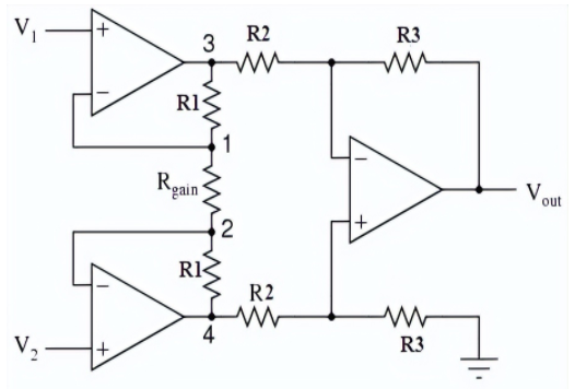
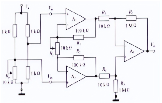
A typical instrumentation amplifier topology uses three operational amplifiers and several resistors. High-precision resistors (0.1% tolerance or better) are used to achieve high CMRR.
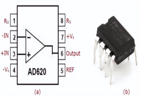
Figure: (a) Pin configuration (b) AD620 instrumentation amplifier package
Instrumentation amplifier circuit requirements
Instrumentation amplifiers are used to amplify low-level signals while rejecting noise and interference. A well-designed instrumentation amplifier should meet the following specifications:
- Limited, accurate, and stable gain: Because instrumentation amplifiers amplify very low-level signals from transducers, a high but finite gain that is accurate and stable is required.
- Easy gain adjustment: Gain should be adjustable within a specified range precisely and easily.
- High input impedance: To avoid loading the signal source, the input impedance should be very high (ideally infinite).
- Low output impedance: The output impedance should be very low (ideally zero) to avoid loading the next stage.
- High CMRR: Sensor outputs transmitted over long lines often contain common-mode signals. A good instrumentation amplifier should amplify only the differential input and reject the common-mode input, so CMRR should ideally be very high.
- High slew rate: A high slew rate is necessary to provide maximum undistorted output voltage swing.
How an instrumentation amplifier works
An instrumentation amplifier consists of two input buffer amplifiers followed by a differential amplifier. The intent is to design an amplifier with high CMRR and large undistorted signal swing.
The amplifier operates as follows:
- The initial amplifiers act as buffers. Each buffer stage uses three resistors; two resistors have equal values except for the gain resistor Rg.
- The voltages at the buffer outputs are labeled Vout1 and Vout2, corresponding to input nodes V1 and V2 at the noninverting inputs.
- The potential drop across the gain resistor is the difference between V1 and V2, which produces a current through Rg. That current flows through the top and bottom resistors, producing the amplified differential outputs.
Instrumentation amplifier formula derivation
The derivation focuses on the amplifier operation and calculating the output voltage gain. The design is divided into two stages: Stage 1 (input buffers) and Stage 2 (differential amplifier). The outputs Vout1 and Vout2 of Stage 1 feed the inputs of the Stage 2 differential amplifier. First find Vout1 and Vout2, then apply the differential amplifier equations.
Stage 1
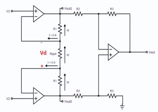
The first stage contains two amplifiers and three resistors connected between inputs V1 and V2 and outputs Vout1 and Vout2.
Assuming ideal op amps with infinite open-loop gain, the voltages at the noninverting and inverting inputs are equal: V- = V+ = V1 for the top amplifier and V- = V+ = V2 for the bottom amplifier. No input current flows into the amplifier inputs, so current from the top R1 must flow through Rg, and that same current continues through the bottom R1. Let Id be the current through Rg, which equals the current through the series resistors.
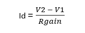
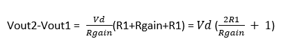
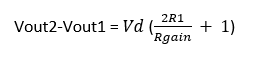
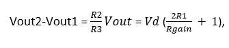
Define Vd = V2 - V1, the differential input. The voltage difference between Vout1 and Vout2 is equal to Id times the appropriate resistor, giving the relation for Vout1 - Vout2 in terms of Vd and the resistor values.
Stage 2 (differential amplifier)
Now that Vout2 - Vout1 is known, it becomes the input to the second stage, which is a differential amplifier. To simplify, first consider a standard differential amplifier and compute its voltage gain.
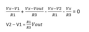
Consider the differential amplifier with inputs V1 and V2 and output Vout. For ideal op amps, V- = V+ = Vx. Apply Kirchhoff's current law at the V- and V+ nodes to derive the equations relating Vout to V1 and V2.
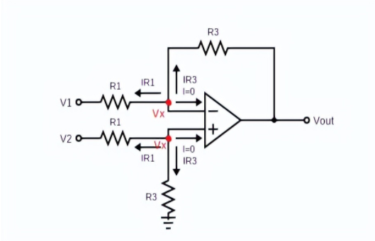

Subtract the two node equations to eliminate Vx and obtain the standard differential amplifier gain expression.
For the original instrumentation amplifier, set the differential amplifier inputs to V1 = Vout1 and V2 = Vout2, and substitute the Stage 1 result for Vout2 - Vout1. The final expression for Vout becomes proportional to the differential input Vd = V2 - V1 multiplied by the overall gain determined by the resistor ratios.
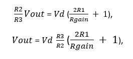
Here Vd = V2 - V1, the differential input.
Instrumentation amplifier circuit examples
1. Instrumentation amplifier built with LM358
U1:A and U1:B are used as voltage buffers to ensure high input impedance. U2:A is used as the differential amplifier. With all differential resistors equal to 10 kΩ, the second stage operates at unit differential gain, so the output voltage is proportional to the voltage difference between pins 3 and 2 of U2:A.
Output voltage formula for this circuit:
Vout = (V2 - V1) (1 + (2R / Rg))
where R = R2 = R3 = R4 = 10 kΩ and Rg = R1 (gain resistor). R and Rg determine the amplifier gain:
Gain = 1 + (2R / Rg)
Example: V1 = 2.8 V, V2 = 3.3 V, R = 10 kΩ, Rg = 22 kΩ.
Vout = (3.3 - 2.8) (1 + (2 × 10 / 22)) = 0.5 × 1.9 = 0.95 V
2. Instrumentation amplifier built with LM324
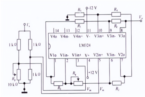
The LM324 integrates four independent op amps in a single package. Using a single quad op amp can reduce performance differences between amplifier channels and simplify power supply arrangements. The basic operating principle remains the same as the three-op-amp instrumentation amplifier.
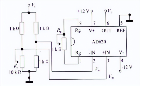
3. Instrumentation amplifier built with AD620
The AD620 is a single-chip instrumentation amplifier that requires only one external gain-setting resistor and a power supply. The circuit is compact and efficient. For the AD620, the gain formula for the shown configuration is:
G = 49.4 kΩ / Rg + 1
4. Instrumentation amplifier built with LM741
An instrumentation amplifier can also be implemented using three general-purpose LM741 op amps with the usual resistor network. The operation is identical to the typical three-op-amp instrumentation amplifier topology.