Introduction
Recently I studied three-phase inverters and summarize the main points here.
1. Circuit topology
The main power topology of a three-phase voltage-source inverter is shown below. The main circuit comprises four parts: the DC supply, six switching devices (complementary conduction), a filter network made of three filter inductors and filter capacitors, and the load, which is three star-connected resistors.
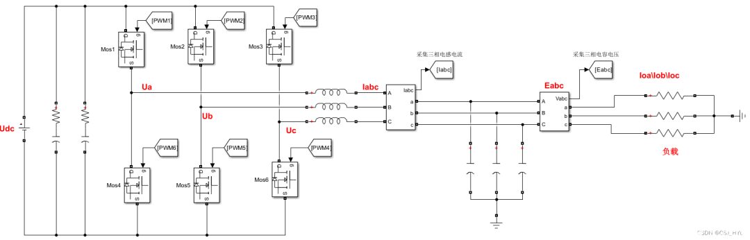
Udc denotes the DC-side voltage. The two capacitors near the DC side are the input filter capacitors. Ua, Ub, Uc denote the midpoint-to-negative DC rail voltages of each inverter leg, i.e. the phase pulse voltages produced by the inverter bridge. Ia, Ib, Ic are the phase currents flowing through the filter inductors. Ea, Eb, Ec denote the capacitor voltages, which are the load voltages. Ioa, Iob, Ioc denote the currents flowing through the load.
2. Mathematical model of the inverter
Developing a mathematical model of the inverter is necessary for controller design. Analysis typically starts from the inductors and capacitors, using KVL and KCL to write circuit equations and derive the model.
2.1 Model in the three-phase stationary abc frame
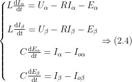
Applying KVL to the three secondary-phase voltage loops yields the equations shown in the figure below.
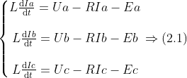
In these equations, R denotes the equivalent series resistance of the phase inductors. Ua, Ub, Uc are the phase voltages for phases a, b, c. Ia, Ib, Ic are the currents through the inductors.
Applying KCL gives the secondary-side current loop equations, shown below.
Combining the KVL and KCL equations provides the inverter model in the three-phase stationary abc frame. While this abc model describes the relationships between voltages and currents, it has multiple inputs and outputs, and the expressions involve many variables, making controller design more complex.
2.2 Model in the alpha-beta (Clarke) frame
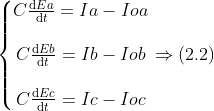
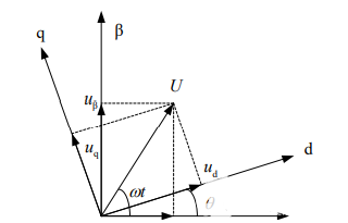
Applying the Clarke transform simplifies the model by converting it to the orthogonal alpha-beta frame. The transform principle is illustrated below.
Because a delta-to-grounded-wye transformer results in zero line-sum on the primary side, there is no zero-sequence component on the primary. Any load imbalance can be treated as a disturbance and is not considered here, so the zero axis is omitted. The corresponding transformation is:
Here, the transformation matrix is:
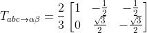
Multiplying by 2/3 is used here because an equal-voltage (voltage-equivalent) transform is applied; the synthesized alpha-beta components can have a maximum magnitude 3/2 times that of the abc stationary components. There is also a power-invariant version of the transform, which is not covered here.
Substituting the Clarke transform into the abc equations yields the alpha-beta frame equations shown below.
The Clarke transform reduces the number of control variables and simplifies the control system. The alpha and beta components are orthogonal and independent, which simplifies control. However, a traditional PI controller tracks AC quantities poorly and may produce steady-state error; since a PI controller does not produce steady-state error for DC quantities, it is common to apply the Park transform to move equation (2.4) into the dq rotating frame.
2.3 Model in the rotating dq frame (Park transform)
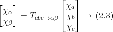
Transforming variables from the two-phase stationary alpha-beta frame to the two-phase rotating dq frame is called the Park transform. The principle is shown below.
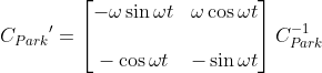
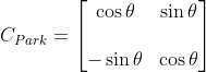
Define the Park transform matrix Cpark. The relationship is:
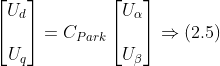
where the transform matrix is:
Combining equations (2.4) and (2.5) yields the dq-frame mathematical model, shown below.
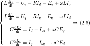
The Park transform moves the model into a rotating reference frame. Since the coordinate frame rotates with the same direction and speed as the reference rotating vector, the transformed quantities appear as DC values in the rotating frame. This simplifies the mathematical model and facilitates control implementation.
3. Equivalent circuit model of the inverter
A transformer-equivalent model for inverters is described in the literature on PWM rectifiers. In that equivalent, the switch duty ratios da, db, dc, da', db', dc' are represented by tap ratios of autotransformers, producing an equivalent transformer model.
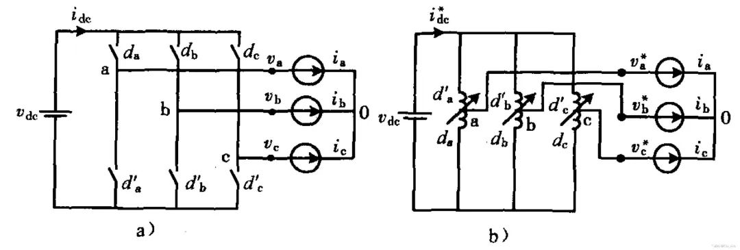
Using the dq-frame model derived earlier, a corresponding dq-frame transformer model can be obtained. This equivalent model helps to visualize and understand the dq-frame mathematical model.
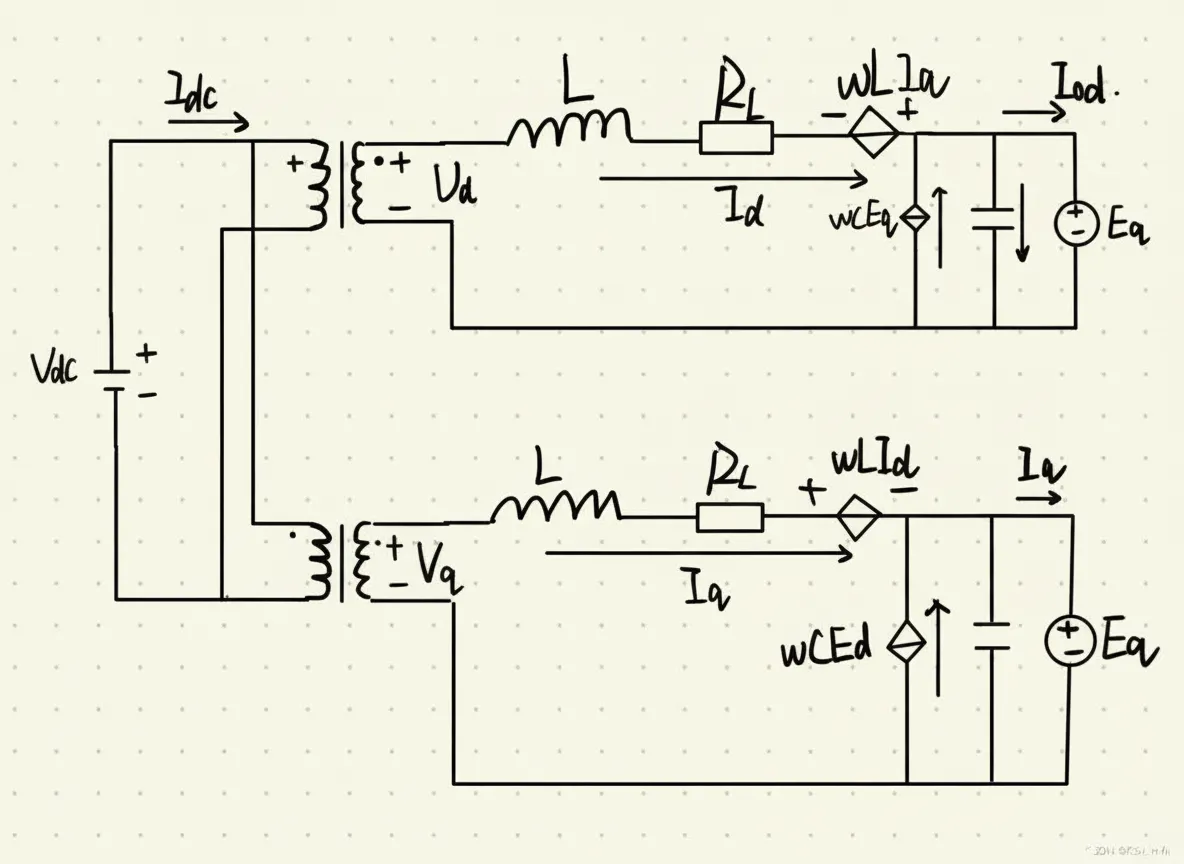
The drawing is approximate and intended for conceptual understanding.
4. Summary
Using Clarke and Park transforms, the inverter model is obtained in different coordinate frames, providing a foundation for controller design. In practice, controller design typically uses the dq-frame model.
The modeling stage here did not consider modulation methods. Modulation is used to generate Ua, Ub, Uc. After deriving the mathematical model and designing the controller, desired Ua, Ub, Uc are obtained; modulation then produces PWM signals to generate the inverter-side voltages and achieve the control objectives.
The coordinate transforms are implemented as matrix operations, so the coordinate conversions are performed using matrix arithmetic.
For example:
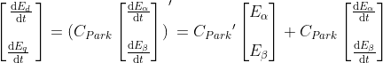
where: