Introduction
Earlier, when discussing solutions to electromagnetic field problems from the oscillator equation, a reader asked how this relates to antennas and how to analyze antennas starting from the oscillator. This article begins a short series on antennas.
There is a saying that only when you can explain a theory to anyone do you truly understand it. I once felt confident about the antenna part because much of my thinking about antennas, oscillator equations, and solutions to electromagnetic field problems started from antennas.
After several attempts I found it still difficult to explain perfectly. Nevertheless, I am confident that a few explanations can give most readers a clear understanding of an antenna’s basic operating process and physical principles.
The approach here is: first analyze charge or carrier motion in a transmission line to clarify the basic forces involved and why a conventional transmission line does not radiate. Next, see how the constraints preventing radiation can be broken, or what conditions permit radiation, and how an antenna is formed. Then focus on the antenna from first principles and finally discuss topics based on those principles.
Note: I mainly discuss antennas from a physical understanding perspective. I use some personal viewpoints and sometimes sacrifice some mathematical rigor for clarity. Please consider the ideas accordingly.
Wave and Standing Wave
First we discuss what signal propagation in a transmission line or circuit looks like. In earlier discussions of electromagnetic field solutions I noted that most problems are understood starting from the oscillator equation. So we briefly recall the basic oscillator equation and its solution.
The general mathematical form of the oscillator equation, ignoring sign conventions, is a second derivative of a function equal to the function times a constant. Its general solution is a combination of exponentials with positive and negative exponents. In some applications the variable may be spatial position, allowing both forward and backward propagation. In the oscillator the variable is time, with a single direction.
Most microwave and electromagnetic field problems are cast into this form and then solved. When this form appears, the solution structure is immediately recognizable and the physical meaning of each quantity can be related back to the oscillator case. The constant in the equation essentially encapsulates material and wave properties.
A sinusoidal steady-state signal in a transmission line satisfies a similar equation. Applying the oscillator solution yields traveling wave solutions. If the position variable z appears with a negative sign it indicates propagation in the +z direction; a positive sign indicates propagation in the ?z direction.
A forward-traveling wave on a conductor has a specific instantaneous charge distribution along the line. Conductors carry charge carriers (electrons), so they are negative charges in reality, but for conceptual clarity both positive and negative charges are used here: a flow of negative charges corresponds to a lack of negative charge (a hole) flowing in the opposite direction, so this representation does not change the analysis results.
Signals reaching the end of a conductor or encountering an impedance change will reflect. For antenna analysis we often assume an open-circuited transmission line end, so there is a significant reverse current. The reverse-traveling wave has the opposite spatial phase sign. When forward and reverse waves coexist the total expression becomes a standing-wave form; the instantaneous carrier distribution is the standing-wave distribution.
That standing-wave distribution follows from superposition of forward and reverse waves. The following sections show a schematic development of how the steady standing distribution arises.
Standing Wave Formation (schematic)
In a schematic sequence, a half-cycle forward signal propagates, then beyond half a cycle the forward signal begins to reflect back. At 0.75 cycle the reflection progresses further, and by one period a steady pattern is established. These diagrams are illustrative and omit transient complexity: before steady-state the transient behavior is complicated and carrier motion is not a simple sinusoidal procession.
We will later try to analyze transient behavior. For now we base subsequent analysis on the standing wave because practical antennas mainly operate under standing-wave conditions. (There are traveling-wave antennas, but the radiation mechanism is the same.)
Earlier we temporarily assumed both positive and negative carriers for intuitive clarity. We can also view carriers as always moving in a single direction before returning at the end. In reality electrons at different positions oscillate locally; once the conceptual picture and physical process are clear, returning to the exact physical description does not change the conclusions.
Standing Waves in Transmission Lines
The previous single-conductor discussion is simplified. Real transmission lines consist of two conductors with opposite polarities, so the normal standing wave in a transmission line takes a form where each conductor supports its own standing-wave set. A quarter-wavelength marker from a location to the end is useful when preparing the monopole analysis.
At the quarter-wavelength position the potentials of the two conductors sum to zero at any time because the amount of positive and negative charge is always equal there, while the current is nonzero. Zero potential and nonzero current imply zero input impedance, i.e., a short circuit. This is the physical reason why a quarter-wave open-circuited stub behaves like a short circuit.
Next we analyze forces at several special instants in the standing-wave cycle.
Force Analysis 1 — Maximum Electric-Field Energy Instant
At this instant every position along the line has zero current because forward and reverse-moving charges are equal in amount, so magnetic-field energy is zero and electric-field energy is maximal.
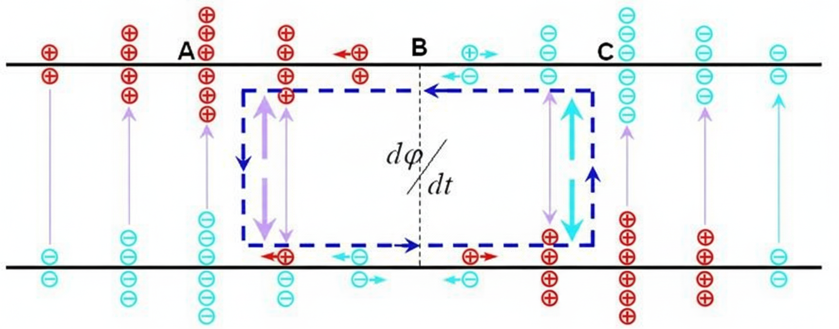
Force and motion: On either side of an electric-field antinode, there are opposite-sign charges and the horizontal electric force is largest. Under this electric force, opposite charges move across the node into the other region. This injection creates current, and the induced magnetic effect (or induced opposing electric field) resists the injection. Initially the injected charge velocity is small while acceleration is maximal, so the magnetic resisting effect is also maximal. As injection continues, velocity increases but acceleration decreases, so the magnetic resisting effect weakens; simultaneously, neutralization of opposite charges reduces the electric force.
Energy: Initially the field between conductors at a point A is strong and energy is stored mainly as electric-field energy. As charges inject into the opposite region, neutralization reduces the field energy at A. Meanwhile the electric force does work against the magnetic resisting effect, converting electric-field energy into magnetic-field energy, until the node regions are electrically neutralized and the stored energy is entirely magnetic at the corresponding location B.
Most of the energy or forces exist between the conductors, but there is also energy outside the conductors. Outside, the forces from the two conductors tend to cancel, so only regions near the conductors have a significant net force; far from the conductors the net force is negligible.
Force Analysis 2 — Maximum Magnetic-Field Energy Instant
At this instant the conductors at every position are electrically neutral, electric-field energy is zero, and magnetic-field energy is maximal.
Force and motion: Electric-field forces are zero and charge velocity (current) is maximal. The moving charges generate a magnetic field that prevents an immediate stop; sudden magnetic-field change would induce a large opposing electric field. The magnetic-induced effect continues charge motion and eventually disrupts the charge balance, leading to accumulation of opposite charges on the node sides. The attractive electric force then resists continued motion. As the amount of opposite charge grows, the electric restoring force increases, and the magnetic influence must do more work to continue motion until it can no longer overcome the electric attraction; at that point the opposite charge amount is maximal and motion stops.
Energy: At this instant the conductors and the space between them reach electrical balance; the system electric-field energy is zero and the current is maximal, so magnetic-field energy is strongest. In the space corresponding to point B the magnetic energy density is maximal. From this point, magnetic forces do work against the electric forces and magnetic energy converts back into electric energy. In this text the term magnetic force refers to the force resulting from the induced electric field produced by changing magnetic fields.
Charge Pairs in the Transmission Line
Because the charges oscillate synchronously, we analyze the behavior by isolating a pair of charges to simplify the discussion.
From Rest to Recombination
Consider a stationary pair of opposite charges located on the two conductors. The combined static field concentrates most field energy between the opposite charges across the gap. When charges start recombining under electrostatic attraction, induced fields appear. The induced magnetic fields from currents in the two conductors are reinforced between the conductors and tend to cancel outside. The induced electric field that resists recombination is also stronger between the conductors and tends to cancel outside.
Horizontal recombination motion reduces the system's electric potential energy. Because the induced fields resist recombination, the diminishing electric energy is converted into increasing magnetic-field energy. The mutual constraint of the two conductors concentrates the magnetic field in a small region between them. Both the static and induced-field energies remain confined between the conductors and cannot diffuse outward. Thus the transmission line's balanced geometry constrains electromagnetic fields and is the reason it does not radiate.
From Recombination to Separation
After recombination, electric energy has been converted mostly into magnetic energy concentrated near the recombined charge pair. The magnetic field tends to separate charges again. Because the magnetic energy is concentrated between the conductors and cannot dissipate or spread, it can drive the charges apart to the pre-recombination configuration but with swapped polarities. Without external perturbation, this pair would oscillate indefinitely at a certain frequency.
In a real transmission line many charge pairs undergo recombination and separation simultaneously. Each recombining pair reduces the electric field between conductors and increases the local magnetic field. Distinguish between force and stored energy: both electric and magnetic fields represent stored potential energy, while the instantaneous electric force magnitude corresponds to the rate of energy conversion. Recombination and separation processes can coexist; the macroscopic result is their net effect, analogous to a phase-change process in materials.
Radiation from Free-Space Charge Pairs
The previous analysis focused on charges constrained by a transmission line. If a pair of opposite charges oscillates in free space, the situation differs because the induced fields are not constrained and can redistribute energy into far-field regions.
Consider a free-space oscillating dipole pair. Initially the two opposite charges have concentrated electric potential energy distributed in space, highest near the charges. When released, recombination converts local electric energy into magnetic energy distributed through space. The induced fields act to reduce field concentration near the charges and strengthen fields farther away, tending to equalize energy distribution in space. After recombination, some magnetic energy is already distributed away from the charge pair and no longer available to restore the charges to the initial separation; that escaped portion constitutes radiation.
If external energy continually supplies the original charge pair to
sustain oscillation, energy is continuously transferred outward and radiated. The near-field region contains the portion of stored energy that remains coupled to the source and can return to it; the far-field contains the radiated portion. The ideal electric dipole model provides formulas for the spatial extent of near and far fields and their energy ratios.
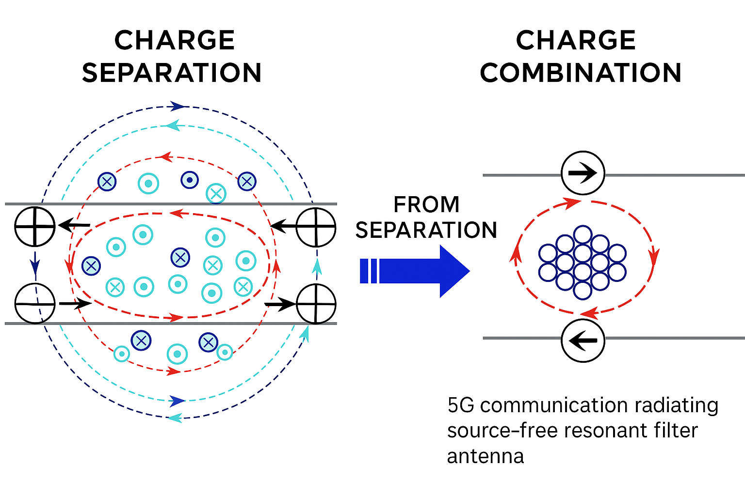
Breaking the Transmission Line Balance — Enabling Radiation
How can one create a space charge pair that radiates? The transmission line geometry constrains fields by mutual cancellation between the two conductors. The simplest way to remove that constraint is to separate the conductors so they no longer overlap their fields. A conceptual illustration shows two conductors spread apart so the mutual cancellation no longer holds.
In that configuration the conductors cannot fully cancel each other’s fields, so oscillating charges produce fields that extend into free space and generate radiation. In practice the field distribution will reconfigure when conductors are moved, but the qualitative conclusion remains: breaking the mutual constraint enables far-field radiation.
If the conductors are only partially separated, some mutual constraint remains, concentrating induced fields near the conductors and weakening the far-field; this explains why antennas with poor radiation efficiency tend to have stronger near fields.
Any conductor supporting oscillating charge pairs can radiate once the constraints that confine fields close to the conductors are reduced. Antennas operate at resonance so that many charge pairs oscillate simultaneously; more charge pairs oscillating concurrently increase the radiated energy per cycle. This is why most antennas are designed to operate in resonant conditions.
Discussion on Radiation
Below are restated points about radiation from other perspectives.
What is radiation: Oscillating charges or alternating currents induce time-varying fields that tend to redistribute energy from concentrated regions to less concentrated regions. The result is enhanced field strength at locations far from the oscillating source compared with static fields, increasing the ability to do work there. That energy transfer into distant regions is radiation.
Why does radiation occur: Energy nonuniformity is inherently unstable. Without external constraints, energy flows spontaneously from higher-energy regions toward lower-energy regions to reach a more uniform distribution. For an oscillating charge in free space, space is effectively infinite so uniformization never completes, and energy keeps transferring outward; consequently radiation continues.
How radiation proceeds: Energy is transferred by the induced fields. The induced fields reduce energy concentration near the source and increase it at farther locations. Electric and magnetic fields are both the medium and carrier of that energy transfer.
Antennas: If a source continually replenishes the concentrated field region so that the near field remains strong despite the outward transfer, the system continuously radiates; this is the antenna function.
Conditions for radiation: Radiation itself is not conditioned; it is an intrinsic property of an oscillating, unbalanced charge system. Preventing radiation requires constraints so that induced fields remain confined near the source. In a two-conductor transmission line these constraints arise from mutual field cancellation between the conductors.
Why static charge pairs do not radiate: Static charge pairs are equilibrium systems held in place by external forces that counteract the spontaneous equalization tendency. Those external forces prevent radiation by suppressing the induced-field-driven energy redistribution.
Implications for Antenna Design
So far the focus has been the radiation mechanism rather than antenna engineering. Many antenna design requirements and concerns become clearer when viewed from the radiation mechanism perspective.
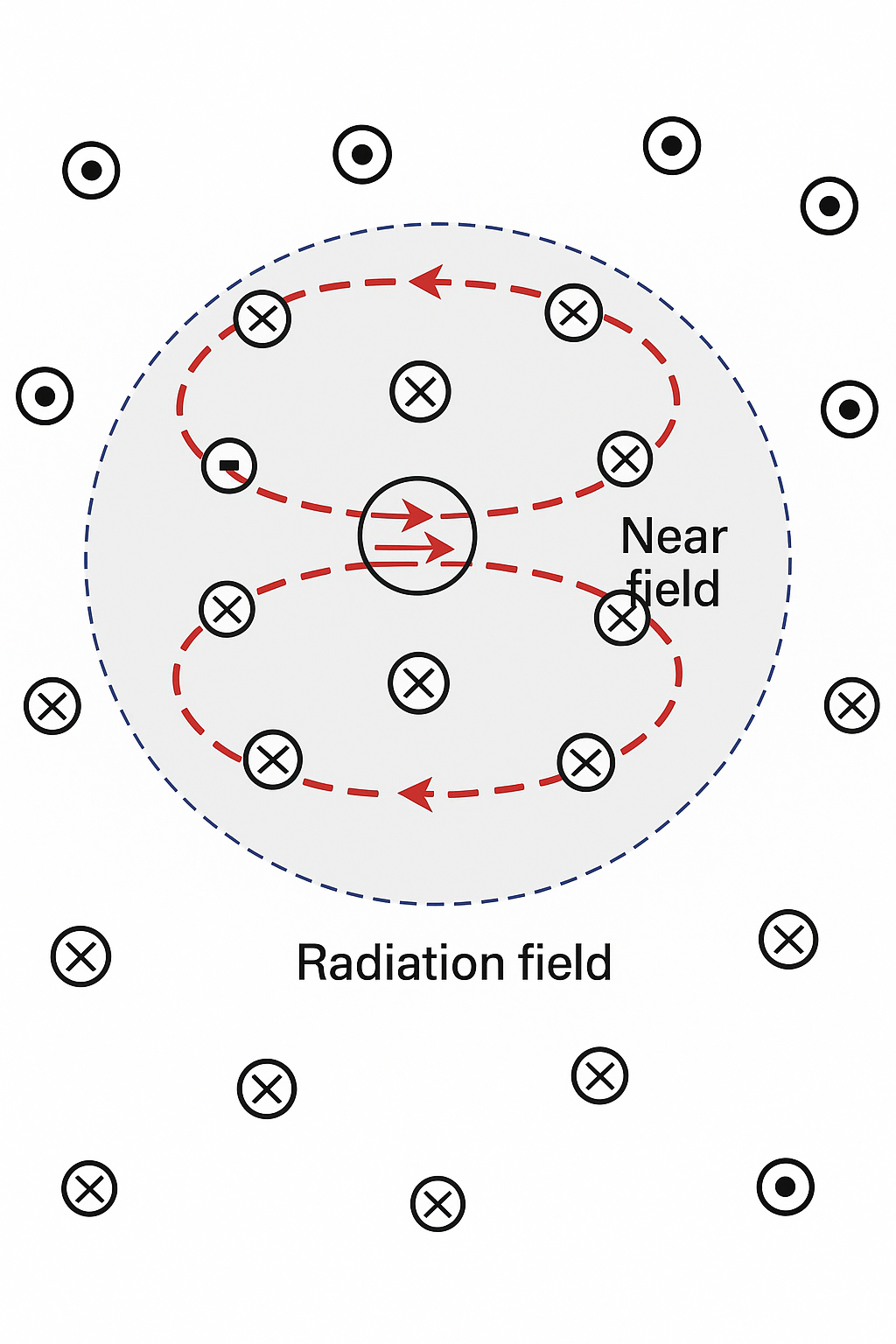
Radiation field considerations: A schematic shows near-field and far-field regions. For an antenna one should maximize the radiated field fraction. How to increase the radiated field?
- Provide open surrounding space to allow field energy to spread.
- Avoid constraints that allow mutual cancellation, such as nearby metal that couples to and confines the field.
- Apply dielectric loading to the radiating region when appropriate to increase the proportion of radiated field.
- Encourage more charge pairs to oscillate simultaneously, i.e., design for resonance, which is why most antennas operate with standing waves.
From the radiation mechanism viewpoint, these practical design aims map directly to physical effects.
Resonance
Before concluding, a brief examination of resonance is warranted because it closely relates to radiation. A simple illustration shows how resonance builds up: the source amplitude may remain constant while the resonant circuit amplitude gradually grows over several cycles until balance is reached.
Initially the resonator amplitude is small. Through successive oscillation cycles, the amplitude increases until, at equilibrium, the energy radiated per cycle equals the energy the source supplies per cycle. At that point the resonance reaches steady state. In this context, R denotes the effective radiation resistance, an equivalent quantity useful for understanding, and should not be confused with the antenna input impedance.
During the resonant buildup every charge pair radiates. As resonance strengthens, more charge pairs participate per cycle and the radiated energy per cycle increases. When the radiated energy per cycle equals the source-provided energy per cycle, resonance is balanced.
Key concepts used here:
- Large numbers of oscillating charge pairs radiate simultaneously; this requires resonance and standing waves so that charges at different positions oscillate in phase.
- Timely replenishment of the near-field weakened by radiation preserves the maximal field gradient for efficient transfer to the far field.
- In non-resonant conditions, the source may not replenish the near-field energy exactly each cycle; this energy then temporarily stores as near-field electric or magnetic energy (capacitance or inductance), reducing the field gradient, weakening induced transfer, and lowering the radiated fraction.