Overview
Obstacle avoidance refers to a mobile robot sensing static or dynamic obstacles along its planned path and updating that path in real time using algorithms so the robot can bypass obstacles and reach its target. Perception of the surrounding environment is the first step for navigation or obstacle avoidance. For obstacle avoidance, a mobile robot must obtain real-time information about nearby obstacles, including size, shape, and position. Common sensors include vision sensors, laser scanners, infrared sensors, and ultrasonic sensors. The following sections summarize their basic principles and typical characteristics.
Common Sensors
Ultrasonic sensors
Ultrasonic sensors measure distance by timing the flight of an ultrasonic pulse and applying d = v t / 2, where d is distance, v is the speed of sound, and t is the round-trip time. Air temperature and humidity affect the speed of sound, so precise measurements must account for environmental variations.
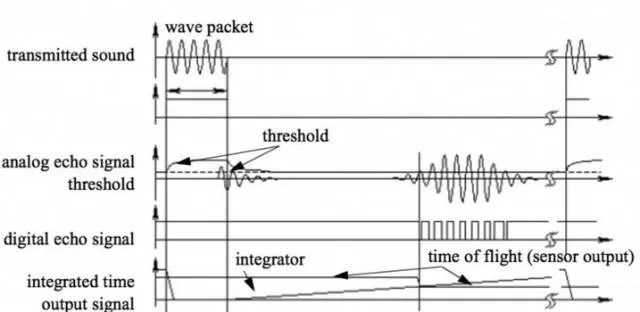
Typically, a piezoelectric or electrostatic transducer emits a burst of ultrasonic pulses in the tens of kHz range. The system detects reflected waves above a threshold and computes distance from measured flight time. Ultrasonic sensors usually have short effective ranges of a few meters and a blind zone on the order of several tens of millimeters. They are low cost, simple to implement, and mature in practice, but they have limitations:
Because sound propagates in a cone, the measured distance corresponds to the nearest object within that cone, not a single point. The measurement period can be long; for example, detecting an object at 3 m requires about 20 ms for a round trip. Different materials reflect or absorb ultrasonic waves differently, and multiple ultrasonic sensors operating simultaneously can interfere with each other. These factors must be considered in system design.
Infrared sensors
Infrared distance sensors commonly use triangulation. An IR emitter projects a beam at a fixed angle; the reflected beam hits a detector (for example, a CCD) at a position related to the target distance via geometric triangulation. When the target is very close, the detected spot can fall outside the detector range and appear invisible; when the target is far, the measured offset becomes small and accuracy degrades. Infrared sensors typically have shorter ranges than ultrasonic sensors and also have a minimum measurable distance. Transparent or near-black objects are difficult or impossible for IR triangulation to detect. Compared with ultrasonic sensors, IR sensors offer higher bandwidth.
Laser scanners (LiDAR)
Common LiDAR systems are based on time-of-flight (ToF) measurement, using d = c t / 2, where c is the speed of light and t is the round-trip time. A LiDAR includes a transmitter and a receiver. Mechanical LiDARs use a rotating mirror mechanism so the beam sweeps a plane and produces distance measurements across that plane.
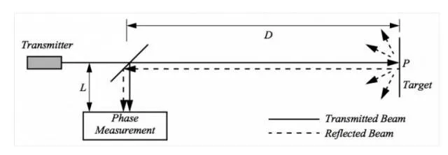
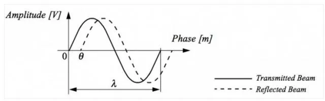
Time-of-flight measurement methods vary. Pulsed lasers measure the direct time interval, requiring very high-precision timing electronics because of the high speed of light, which increases cost. Frequency-modulated continuous-wave (FMCW) LiDAR transmits a chirped signal and measures the beat frequency between transmitted and received signals to infer distance.
LiDARs can reach ranges of tens to hundreds of meters with high angular resolution, often sub-degree, and high distance accuracy. Measurement confidence decreases roughly with the square of the received signal amplitude, so dark or distant objects yield lower confidence than bright, close objects. Transparent materials like glass are problematic. LiDAR systems tend to be complex and costly. Low-end LiDARs may use triangulation with limited range and lower accuracy but can suffice for indoor SLAM or outdoor obstacle avoidance at low speed.
Vision sensors
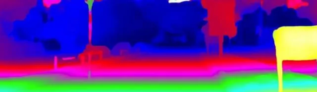
Computer vision solutions include stereo vision, ToF depth cameras, and structured light depth cameras. Depth cameras produce both an RGB image and a depth map. Active depth sensors (ToF or structured light) perform poorly in strong ambient light because they rely on active illumination; thus, passive stereo vision is often better for outdoor environments exposed to sunlight.
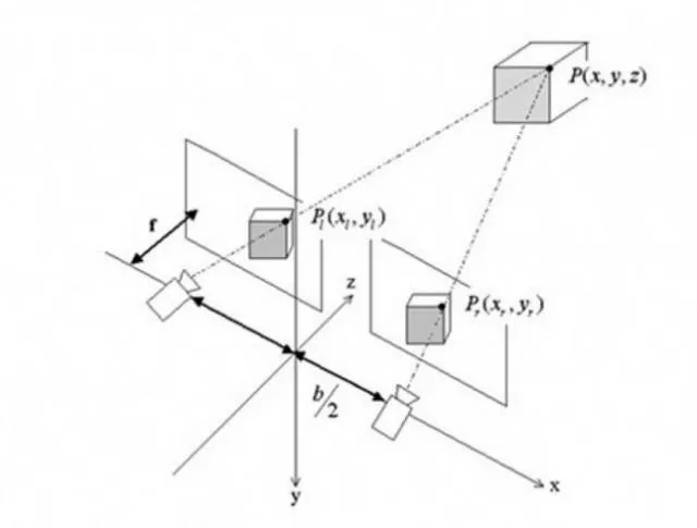
Stereo vision measures depth by triangulation: two cameras with a known baseline observe the same world point P at different pixel coordinates; triangulation yields the distance. Unlike structured light, which emits a known pattern, stereo algorithms match image features such as SIFT or SURF to compute correspondences, typically producing a sparse depth map.
For robust obstacle avoidance, dense point clouds are preferable to sparse feature sets. Dense stereo matching algorithms fall into two categories: local methods using neighborhood pixel information, and global methods using information from the entire image. Local methods are faster; global methods tend to be more accurate. Dense stereo outputs provide scene depth similar to LiDAR point clouds but with richer appearance information. Vision systems are much cheaper than LiDAR but require more computation and usually offer lower absolute depth precision. In many practical applications the depth accuracy is sufficient, and real-time performance can be achieved on embedded platforms such as NVIDIA TK1 and TX1.
From continuous camera frames, it is also possible to estimate the motion of objects in the scene and build motion models to predict their direction and speed, which aids trajectory planning and obstacle avoidance.
Sensor Fusion Strategy
Each sensor has strengths and weaknesses. In real systems, multiple sensor modalities are typically combined to maximize the probability of correctly detecting obstacles across different environments and object materials. A common approach is to use a primary sensing modality (for example, stereo vision) supplemented by additional sensors such as LiDAR, ultrasonic, or infrared to cover blind spots and increase robustness, providing near-360-degree awareness around the robot.
Common Obstacle Avoidance Algorithms
Assume the robot already has a navigation planner that provides a planned trajectory. The obstacle avoidance algorithm updates the trajectory in real time when sensors detect obstacles so the robot can bypass them while continuing toward the goal.
Bug algorithms
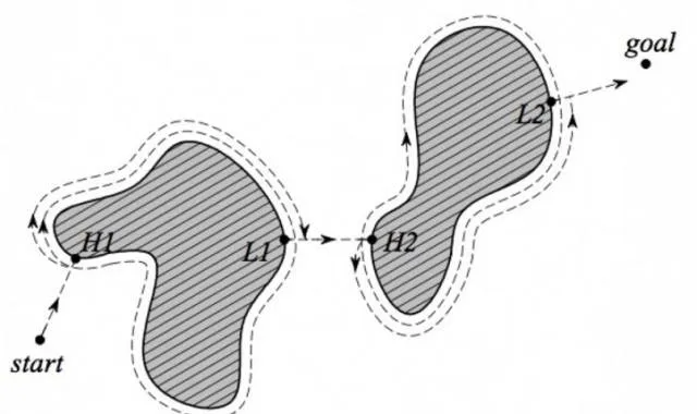
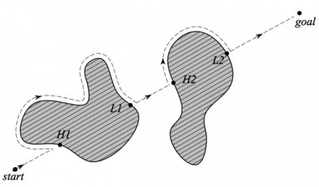
Bug algorithms are simple. After detecting an obstacle, the robot follows the obstacle boundary to bypass it. Examples include Bug1, where the robot completely circumnavigates the object and then departs from the point closest to the goal. Bug1 is guaranteed to reach the goal but is inefficient. Bug2 improves efficiency by following the obstacle boundary only until the robot can move directly toward the goal again, producing shorter paths. Variants such as TangentBug exist. Bug algorithms are easy to implement but do not account for robot kinematics or dynamics, reducing reliability in complex environments.
Potential field method
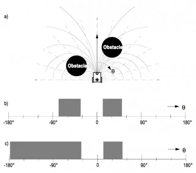
Potential field methods treat the robot as a point moving in a potential field: the goal exerts an attractive potential while obstacles create repulsive potentials. These forces sum to guide the robot smoothly toward the goal while avoiding known obstacles. When new obstacles are detected, the potential field is updated and the path replanned.
Extensions add additional fields such as transport and task fields to account for relative orientation and velocity between robot and obstacles. Transport fields increase repulsion when the robot is heading toward an obstacle and reduce it when moving parallel. Task fields ignore obstacles that do not affect near-term potential based on current velocity, producing smoother paths. Potential field methods have theoretical issues like local minima and oscillation, but they are easy to implement and can work well in practice with appropriate enhancements.
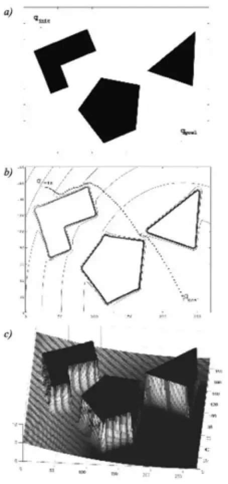
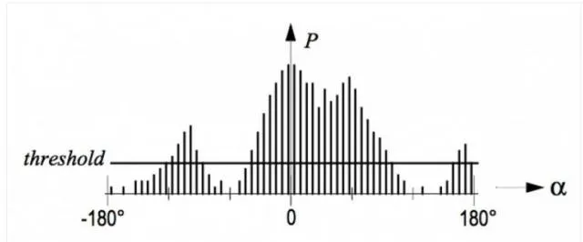
Vector Field Histogram (VFH)
VFH constructs a local polar occupancy histogram around the robot from recent sensor data represented on a grid. The algorithm identifies sufficiently wide free sectors and evaluates a cost function for each candidate sector, then selects the sector with minimum cost. The cost is a weighted sum of factors such as goal direction, current robot heading, and previously chosen directions. Weight tuning adjusts the robot's preference. VFH+ introduces robot kinematic constraints so trajectories that are blocked under the robot's actual motion model are discarded. For agile platforms such as differential-drive robots, such constraints may be less restrictive.
Learning and fuzzy methods
Neural network approaches can be trained to map from the robot state, velocity, and sensor inputs to desired next heading or motion commands. Fuzzy logic approaches encode expert heuristics as fuzzy rules in a fuzzy controller; for example: if an obstacle is detected far right-front, turn slightly left; if an obstacle is close right-front, slow down and turn left more. These methods can provide adaptive, heuristic-based behavior but require careful training or rule design.
Practical Challenges
Sensor failure and limitations
No sensor is perfect. Transparent surfaces like glass can cause IR, LiDAR, or vision systems to miss obstacles, so ultrasonic sensors may be needed for robust detection. Combining multiple sensors with cross-validation and data fusion improves reliability.
Other failure modes include mutual interference between sensors. For example, ultrasonic arrays may interfere if multiple sensors emit simultaneously, causing cross-reception and erroneous readings. Sequencing sensors reduces interference but increases sampling latency because ultrasonic measurements have relatively long cycles. Hardware and algorithm design should minimize sampling delay and inter-sensor crosstalk.
Electromagnetic interference from motors and drivers can corrupt analog sensor readings. Proper isolation between motors, drivers, sensor acquisition circuitry, and power/communication lines is necessary to ensure stable operation.
Algorithm design
Many obstacle avoidance algorithms do not fully consider the robot's kinematic and dynamic constraints. A planned trajectory may be infeasible to execute or may require aggressive maneuvers that the actuators cannot provide. Algorithm design must account for the platform's motion capabilities and actuator limits.
During operation, obstacle avoidance is often the highest-priority task to prevent harm to people or the robot. The avoidance module should have the highest execution priority and meet real-time performance requirements.
In summary, obstacle avoidance is a specialized, local, and dynamic aspect of autonomous navigation. It places stricter requirements on real-time performance and reliability than global planning, and these factors should inform hardware and software architecture decisions.
Multi-robot Cooperative Obstacle Avoidance
Multi-robot cooperative strategies remain an active research area in SLAM and obstacle avoidance. A common approach is for each robot to maintain a local dynamic map while sharing a relative static global map. When robots approach one another, they merge their local dynamic maps to expand situational awareness. For example, a rear robot can contribute information about areas behind a front robot, enabling complete local dynamic coverage for obstacle avoidance.
Key issues include how to share local maps and handle communication constraints. Combining local windows on the relative global map allows fusion and coordination, but multi-robot cooperation must account for transmission latency and bandwidth limits; local operations remain faster since they run on-board.
Testing Metrics and Standards
There is no single industry-wide standard for obstacle avoidance testing. Typical evaluation metrics include success rate in avoiding single or multiple obstacles, performance with static versus dynamic obstacles, path optimality, trajectory smoothness, and perceived behavior quality.
Among these metrics, the fundamental measure is success rate: whether the robot avoids collisions across object materials and motion patterns, including dynamic objects such as people wearing different clothing, and under varying environmental conditions such as lighting. Success rate is the most critical metric for obstacle avoidance performance.