Preface
After the release of YOLOv6, the original authors of the YOLO series released YOLOv7.
YOLOv7's main contributions include:
- Model re-parameterization. YOLOv7 integrates re-parameterization into the network architecture; this idea first appeared in RepVGG.
- Label assignment strategy. The label assignment combines YOLOv5's cross-grid search with YOLOX's matching strategy.
- ELAN efficient network architecture. A new architecture focused on efficiency.
- Training with auxiliary heads. An auxiliary-head training method that increases training cost to improve accuracy without affecting inference time, since auxiliary heads are only used during training.
1. What is YOLOv7?
YOLO is a representative one-stage object detection algorithm that uses deep neural networks to perform object recognition and localization at high speed, enabling real-time applications.
YOLOv7 is the latest iteration in the YOLO series, improving both accuracy and speed compared with earlier YOLO versions.
Understanding YOLO is an essential step for researching object detection algorithms.
2. Network Architecture
Overview of the architecture
The architecture overview:
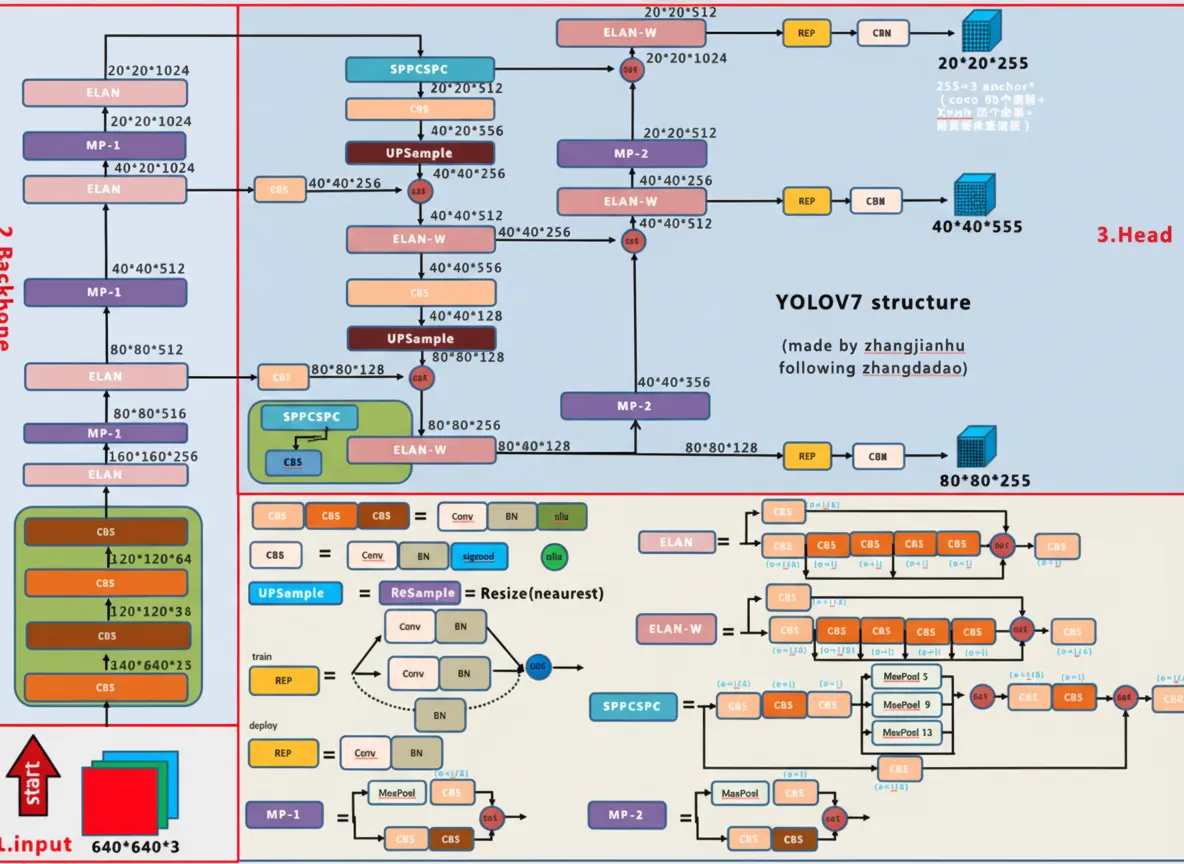
CBS module
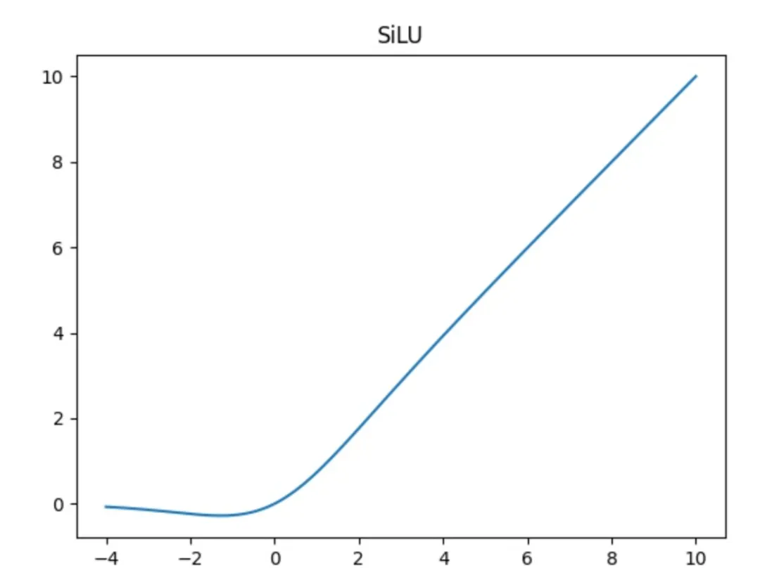
The CBS module consists of a convolution layer (Conv), a batch normalization layer (BN), and a SiLU activation.
SiLU is a variant of the Swish activation. The formulas are:
silu(x) = x * sigmoid(x)
swish(x) = x * sigmoid(beta * x)
In the architecture diagram, three CBS colors indicate different kernel sizes and strides:
- The lightest color represents a 1x1 convolution with stride 1, mainly used to change channel count.
- The medium color represents a 3x3 convolution with stride 1, used for feature extraction.
- The darkest color represents a 3x3 convolution with stride 2, used for downsampling.
CBM module
The CBM module is similar to the CBS module. It contains a Conv layer, a BN layer, and a sigmoid activation. The convolution is 1x1 with stride 1.
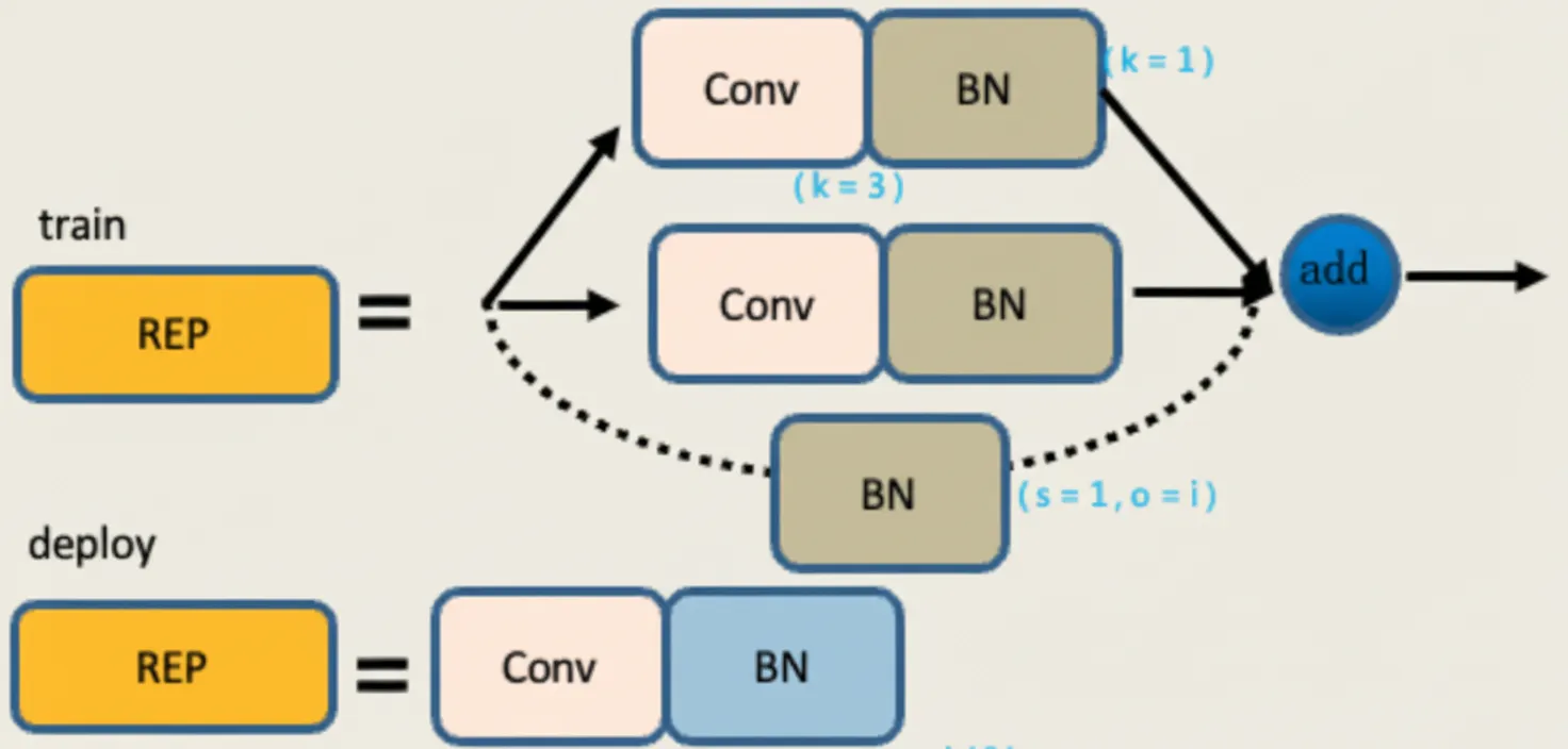
REP module
The REP module has two modes: train and deploy.
In the training mode there are three branches:
- The top branch is a 3x3 convolution for feature extraction.
- The middle branch is a 1x1 convolution for feature smoothing.
- The bottom branch is an Identity branch with no convolution.
The outputs of the three branches are summed together.
In deploy mode the module is converted into a single 3x3 convolution with stride 1 via re-parameterization. The 1x1 convolution and the Identity branch are both converted to equivalent 3x3 kernels, and the weights are merged by matrix addition, producing one 3x3 convolution whose weights equal the sum of the three branches.
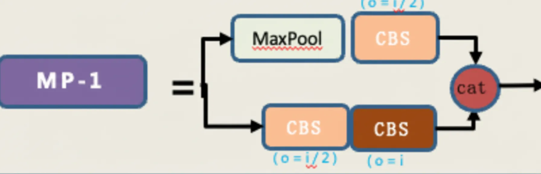
MP module
The MP module has two branches and performs downsampling.
- The first branch applies max pooling for downsampling, followed by a 1x1 convolution to change channels.
- The second branch applies a 1x1 convolution to change channels, then a 3x3 convolution with stride 2 for downsampling.
The two branch outputs are added together to produce the downsampled result.
ELAN module
The ELAN module is an efficient network block that controls the shortest and longest gradient paths so the network can learn more features and improve robustness.
ELAN has two branches:
- The first branch uses a 1x1 convolution to change channel count.
- The second branch first applies a 1x1 convolution then four 3x3 convolution modules for feature extraction. The four resulting features are concatenated or summed to obtain the final output.
ELAN-W module
The ELAN-W module is similar to ELAN. The difference is the number of outputs selected in the second branch for the final aggregation: ELAN selects three outputs, while ELAN-W selects five outputs for the final addition.
UPSample module
The UPSample module performs upsampling using nearest-neighbor interpolation.
SPPCSPC module
The SPP component increases the receptive field to make the network adapt to different input resolutions. It uses max pooling with multiple kernel sizes to capture different receptive fields.
In one branch, multiple max pools are applied with kernel sizes such as 5, 9, 13, and 1, representing different receptive fields for different object sizes. This helps the network distinguish between large and small objects in the same image.
The CSP structure splits features into two parts: one part receives regular processing, while the other part goes through the SPP structure. The two parts are then merged, which reduces computation while maintaining or improving accuracy.