Overview
This article reviews the theory behind diffusion models and demonstrates how to generate images with diffusion models in PyTorch. Diffusion models have become one of the most notable developments in machine learning in recent years. Here we cover the essential concepts and practical steps needed to implement and run image diffusion models.
What Is a Diffusion Model
Diffusion models are generative models that corrupt training data by progressively adding Gaussian noise, then learn to reverse that noise process to recover data. After training, the learned denoising process can be applied to randomly sampled noise to generate new data.
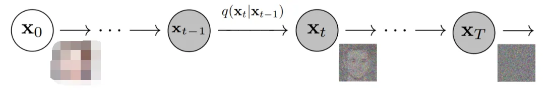
More specifically, diffusion models are latent-variable models that use a fixed Markov chain to map data into latent space. The chain gradually adds noise to the data, producing latent variables with the same dimensionality as x0. The image below illustrates such a Markov chain.
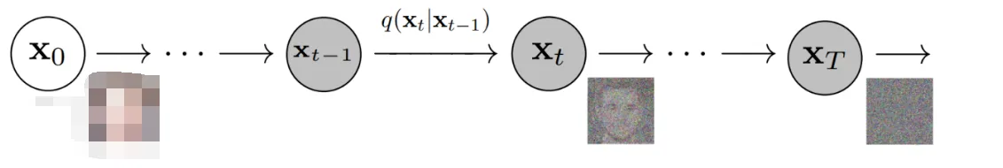
Eventually the image becomes near-pure Gaussian noise. The training objective is to learn the reverse process. By traversing the chain backward we can generate new samples.
Advantages of Diffusion Models
Diffusion models have seen rapid research growth. Inspired by non-equilibrium thermodynamics, they currently produce state-of-the-art image quality in many settings.
Besides high image quality, diffusion models avoid adversarial training, which is known to be difficult. They also offer scalability and parallelism advantages for training efficiency.
Although the results can seem striking, they are grounded in careful mathematical design and hyperparameter choices; best practices continue to evolve in the literature.
Diffusion Models — Details
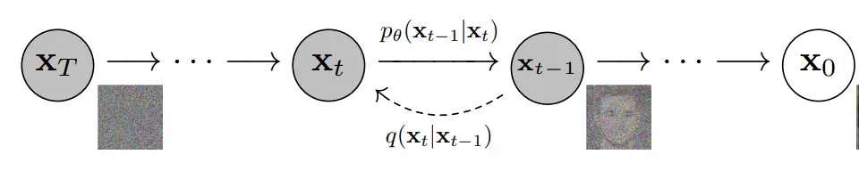
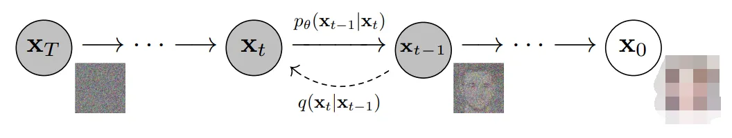
As noted, a diffusion model consists of a forward (diffusion) process and a reverse (denoising) process. The forward process progressively adds noise to data; when noise levels are small, the forward transitions can be modeled as conditional Gaussians. With the Markov assumption the forward process is parameterized as a simple Gaussian chain.

The variance schedule is either learned or fixed; with a suitable schedule and large T the terminal distribution approaches an isotropic Gaussian.
Under the Markov assumption the joint distribution over latents factorizes as a product of Gaussian conditionals. The key is learning the reverse process: starting from pure Gaussian noise the model learns a parameterized joint distribution formed by reversing the chain, where the time-dependent Gaussian parameters are learned. The reverse conditional at time t depends only on the adjacent time step:


Training
Diffusion models are trained by finding reverse Markov transitions that maximize the likelihood of the training data. In practice training is equivalent to minimizing a variational bound on the negative log-likelihood.

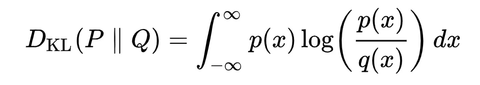
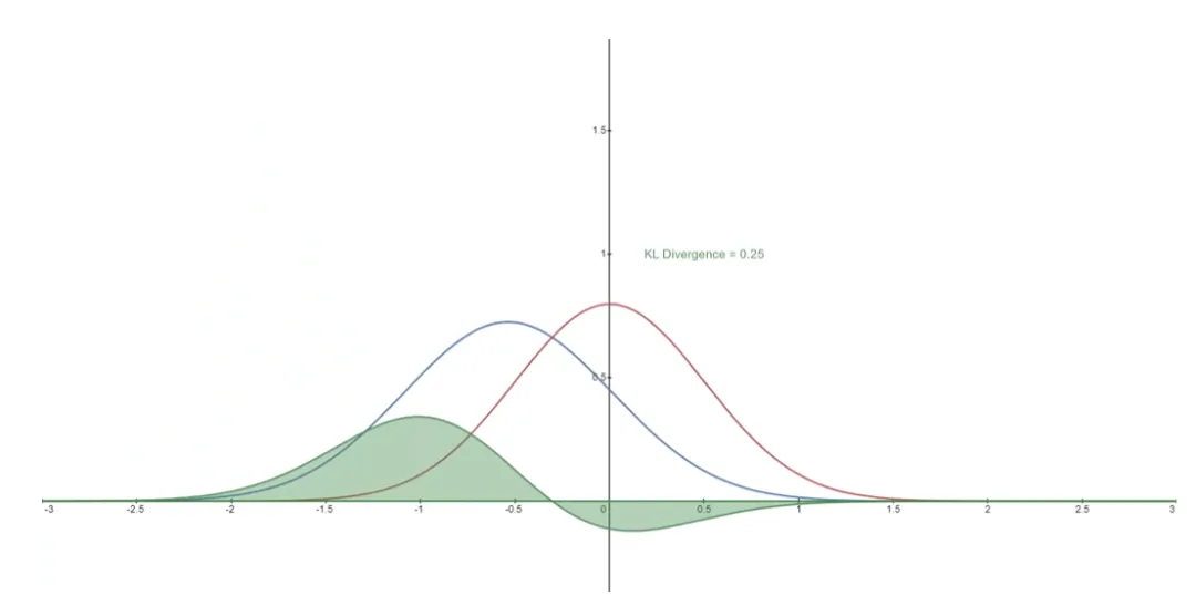
The objective can be rewritten using Kullback-Leibler (KL) divergences. KL divergence measures the difference between a distribution P and a reference distribution Q. Rewriting the objective in terms of KL divergences is useful because the Markov chain transition distributions are Gaussian and the KL between Gaussians has a closed form.
What is KL divergence?
The KL divergence for continuous distributions is given by the standard mathematical expression. The integrand shows how the divergence accumulates pointwise; the total area under that curve equals the KL divergence between P and Q.
Rewriting the objective in KL form
The training objective can be rearranged into a sum of KL terms. By conditioning forward-process posteriors on later latents we obtain tractable closed-form expressions for each KL term, since they compare Gaussian distributions.

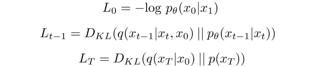
Conditioning the forward-process posterior yields Gaussian comparisons that can be computed exactly rather than estimated by Monte Carlo.
Model Choices
With the objective defined, practical choices remain for implementing a diffusion model. For the forward process the main choice is the variance schedule, which typically increases over time. For the reverse process one usually parameterizes Gaussian conditionals and selects a model architecture—only requirement is matching input and output dimensions.
Forward process and variance schedule
The variance schedule can be set as a fixed time-dependent sequence. Common schedules include linear or geometric progressions. With a fixed schedule, these variances are treated as constants during training and can be ignored when optimizing model parameters.

Reverse process parameterization
The reverse Markov transitions are modeled as Gaussians. We must specify the functional forms of the time-dependent mean and variance. A common, simple choice is to model the reverse conditional as a product of independent Gaussians with shared variance per time step. Those variances are taken from the forward-process schedule.

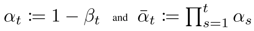
Given this form, the reverse conditional mean can be expressed as a linear combination of xt and x0 that depends on the variance schedule. Rather than directly parameterizing the posterior mean, it has been found more effective to train the model to predict the added noise at each time step. Specifically, let the model predict epsilon:
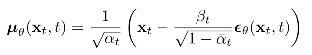
This leads to a simplified loss function that empirically yields more stable training and better results:

Researchers have also noted connections between diffusion formulations and score-matching generative models based on Langevin dynamics. Diffusion-based and score-based models can be viewed as complementary formulations of the same underlying generative principles.
Network Architecture
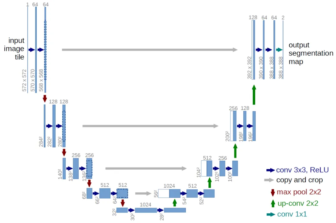
The simplified loss trains a model that maps an input tensor to an output tensor of the same shape. Given this constraint, image diffusion implementations commonly use U-Net-like architectures.
Discrete Decoder for Final Step
The reverse chain consists of many Gaussian conditionals. At the end we must map continuous outputs to discrete pixel values. The standard approach is to treat the final reverse step as an independent discrete decoder. By assuming independence across data dimensions we evaluate the probability of each quantized pixel value given the corresponding Gaussian at t=1.

If images are encoded as integers 0..255 and linearly scaled to [-1,1], the continuous range for a pixel value x is [x-1/255, x+1/255]. The probability of discrete pixel value x is the area under the corresponding univariate Gaussian on that interval.

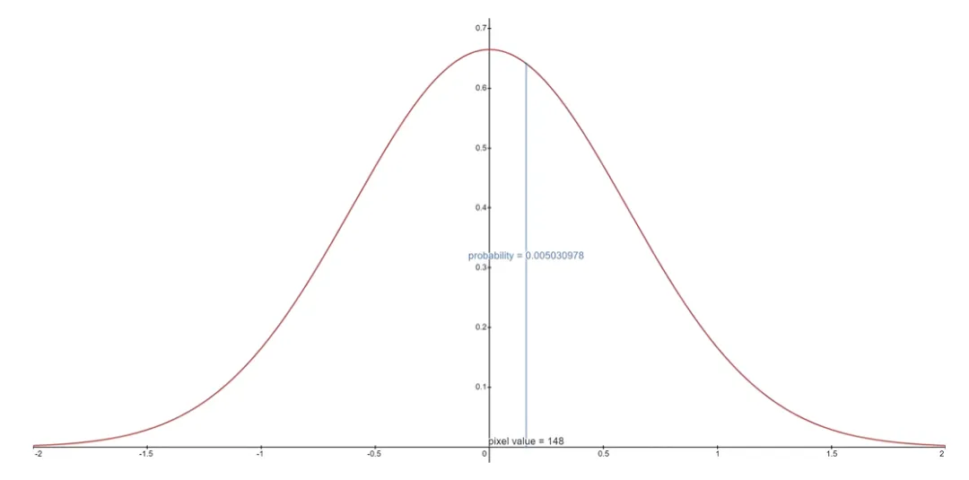
For an entire image, the log-likelihood is the sum over pixels of these per-pixel log-probabilities.


Final Objective
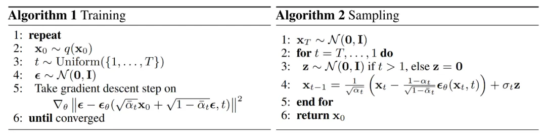
Empirically, predicting the noise at each time step yields the best results. The final training objective used in practice is the simplified noise-prediction loss:

The training and sampling algorithms for the diffusion model are summarized below.
Summary
- Diffusion models are parameterized as Markov chains: latents depend only on neighboring time steps.
- Transitions in the Markov chain are Gaussian. The forward process uses a variance schedule; reverse parameters are learned.
- For large T the forward process approaches an isotropic Gaussian.
- Variance schedules are often fixed but can be learned; geometric schedules may outperform linear ones in some cases.
- Architecturally flexible: any network with matching input and output shapes can be used, commonly U-Net-like networks.
- Training maximizes data likelihood, corresponding to minimizing a variational upper bound on negative log-likelihood.
- Nearly all terms reduce to KL divergences between Gaussians and are computable in closed form.
- Predicting the noise component at each time step with a simplified loss yields stable and strong results.
- A discrete decoder is used for the final reverse step to produce pixel log-likelihoods.
With this overview, the next section shows how to use diffusion models in PyTorch.
Diffusion Models in PyTorch
There are implementations available for diffusion models. A straightforward option in PyTorch is the denoising-diffusion-pytorch package, which implements the image diffusion model described above. Install it with pip:
pip install denoising_diffusion_pytorch
Minimal Example
First import the required packages:
import torchfrom denoising_diffusion_pytorch import Unet, GaussianDiffusion
Define a U-Net model. The dim parameter sets the number of feature channels before the first downsampling; dim_mults scales the channels at each downsampling stage.
model = Unet( dim = 64, dim_mults = (1, 2, 4, 8))
Define the diffusion model by passing the U-Net and other parameters such as image size, number of timesteps, and loss type.
diffusion = GaussianDiffusion( model, image_size = 128, timesteps = 1000, # number of steps loss_type = 'l1' # L1 or L2)
Train on a batch (here we use random tensors as an example), compute the loss from the diffusion object and backpropagate:
training_images = torch.randn(8, 3, 128, 128)loss = diffusion(training_images)loss.backward()
After training, generate images with the sample method. Here we sample 4 images; with random training data the outputs will be noise.
sampled_images = diffusion.sample(batch_size = 4) 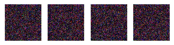
Training on a Custom Dataset
The denoising-diffusion-pytorch package provides a Trainer class to train on a dataset directory. Replace 'path/to/your/images' with the dataset path and set image_size appropriately. Note that Trainer requires PyTorch with CUDA enabled for GPU training.
from denoising_diffusion_pytorch import Unet, GaussianDiffusion, Trainermodel = Unet( dim = 64, dim_mults = (1, 2, 4, 8)).cuda()diffusion = GaussianDiffusion( model, image_size = 128, timesteps = 1000, # number of steps loss_type = 'l1' # L1 or L2).cuda()trainer = Trainer( diffusion, 'path/to/your/images', train_batch_size = 32, train_lr = 2e-5, train_num_steps = 700000, # total training steps gradient_accumulate_every = 2, # gradient accumulation steps ema_decay = 0.995, # exponential moving average decay amp = True # turn on mixed precision)trainer.train()
Below is an example GIF showing denoising from multivariate Gaussian noise to MNIST digits, illustrating the reverse diffusion process.