Overview
This is a collection of Python code for robotics algorithms, with an emphasis on autonomous navigation algorithms.
Environment requirements
- Python 3.6.x
- numpy
- scipy
- matplotlib
- pandas
- cvxpy 0.4.x
How to use
- Install the required libraries.
- Clone the repository.
- Run the Python scripts in each directory.
Localization
3.1 Extended Kalman Filter (EKF) localization
This example implements sensor fusion localization using the Extended Kalman Filter (EKF). The blue line is the true path, the black line is the dead reckoning trajectory, green dots are position observations (e.g., GPS), and the red line is the EKF estimated path. Red ellipses show the EKF estimated covariance.
Further reading:
Probabilistic Robotics
http://www.probabilistic-robotics.org/
3.2 Unscented Kalman Filter (UKF) localization
This example implements sensor fusion localization using the Unscented Kalman Filter (UKF). The lines and markers have the same meaning as in the EKF example.
Further reading:
Discriminatively Trained Unscented Kalman Filter for Mobile Robot Localization
https://www.researchgate.net/publication/267963417_Discriminatively_Trained_Unscented_Kalman_Filter_for_Mobile_Robot_Localization
3.3 Particle Filter (PF) localization
This example implements sensor fusion localization using a particle filter (PF). The blue line is the true path, the black line is dead reckoning, green dots are position observations (e.g., GPS), and the red line is the PF estimated path. The algorithm assumes the robot can measure distances to landmarks such as RFID, which are used by the PF.
Further reading:
Probabilistic Robotics
http://www.probabilistic-robotics.org/
3.4 Histogram filter localization
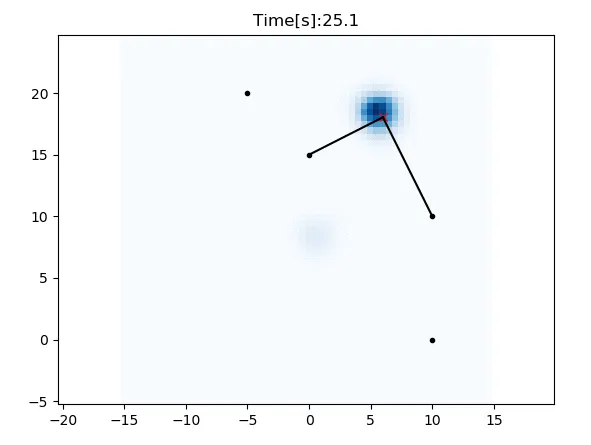
This example demonstrates two-dimensional localization using a histogram filter. The red cross is the true position, black dots are RFID landmark positions, and blue cells show the filter probability. In this simulation, x and y are unknown while yaw is known. The filter integrates velocity inputs and distance observations from RFID for localization. No initial position is required.
Further reading:
Probabilistic Robotics
http://www.probabilistic-robotics.org/
Mapping
4.1 Gaussian grid mapping
Example of two-dimensional Gaussian grid mapping.
4.2 Ray casting grid mapping
Example of two-dimensional ray casting grid mapping.
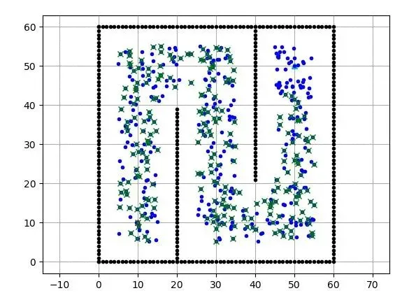
4.3 k-means object clustering
Example of two-dimensional object clustering using k-means.
4.4 Circular fitting for object shape recognition
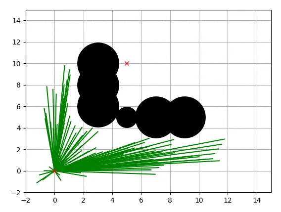
Example of object shape recognition using circle fitting. The blue circle is the true object shape, red crosses are points observed by a distance sensor, and the red circle is the estimated object shape from circle fitting.
SLAM
Examples of simultaneous localization and mapping (SLAM).
5.1 Iterative Closest Point (ICP) matching
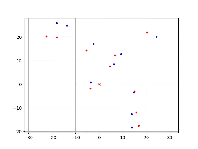
This example uses a closed-form solution to perform two-dimensional ICP matching. It computes rotation and translation between two point sets.
Further reading:
Introduction to robot motion: Iterative Closest Point algorithm
https://cs.gmu.edu/~kosecka/cs685/cs685-icp.pdf
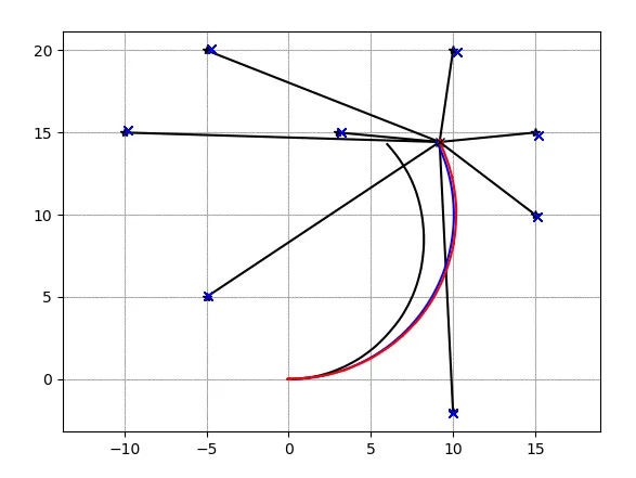
5.2 EKF SLAM
This is an EKF-based SLAM example. The blue line is the true path, the black line is dead reckoning, the red line is the EKF SLAM estimated path, and green crosses are estimated landmarks.
Further reading:
Probabilistic Robotics
http://www.probabilistic-robotics.org/
5.3 FastSLAM 1.0
Feature-based SLAM example using FastSLAM 1.0. Blue line is the true path, black line is dead reckoning, red line is FastSLAM estimate. Red dots are particles, black dots are landmarks, blue crosses are estimated landmark positions.
Further reading:
Probabilistic Robotics
http://www.probabilistic-robotics.org/
5.4 FastSLAM 2.0
Feature-based SLAM example using FastSLAM 2.0. Animation semantics are the same as for FastSLAM 1.0.
Further reading:
Probabilistic Robotics
http://www.probabilistic-robotics.org/
Tim Bailey SLAM simulations
http://personal.acfr.usyd.edu.au/tbailey/software/slam_simulations.htm
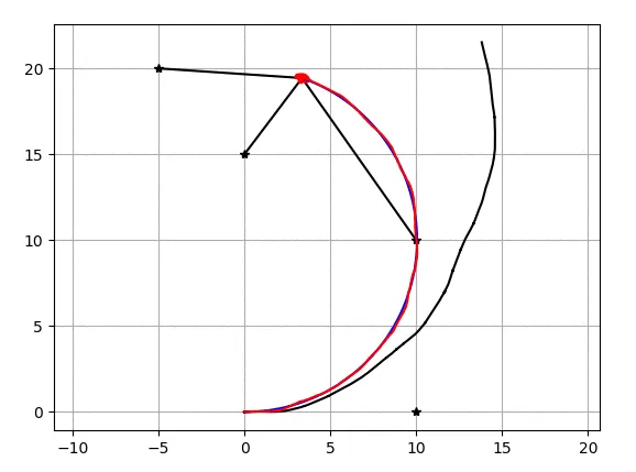
5.5 Graph-based SLAM
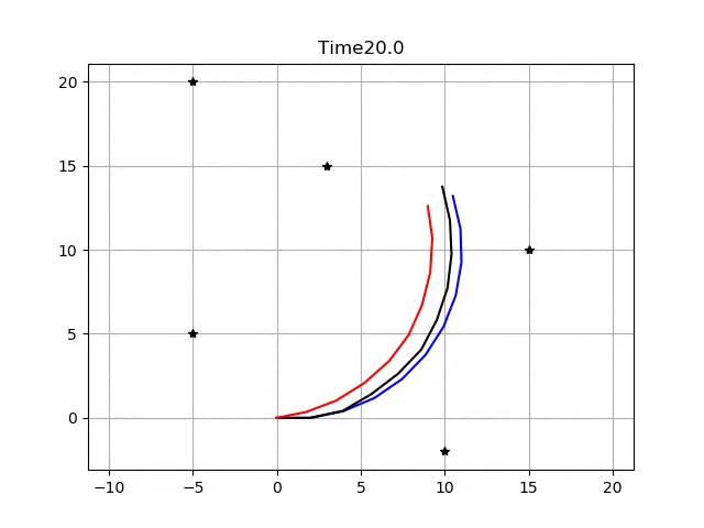
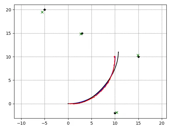
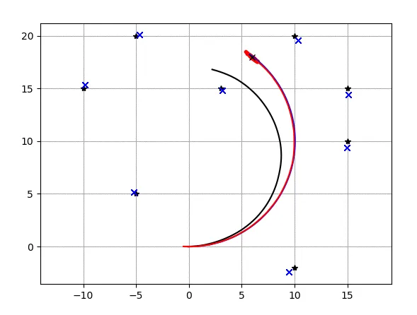
Example of graph-based SLAM. Blue line is the true path, black line is dead reckoning, red line is graph-based SLAM estimate. Black stars are landmarks used to form graph edges.
Further reading:
Introduction to graph-based SLAM
http://www2.informatik.uni-freiburg.de/~stachnis/pdf/grisetti10titsmag.pdf
Path planning
6.1 Dynamic Window Approach
Example of two-dimensional navigation using the Dynamic Window Approach.
Further reading:
Using the Dynamic Window Approach to avoid collisions
https://www.ri.cmu.edu/pub_files/pub1/fox_dieter_1997_1/fox_dieter_1997_1.pdf
6.2 Grid-based search
Dijkstra
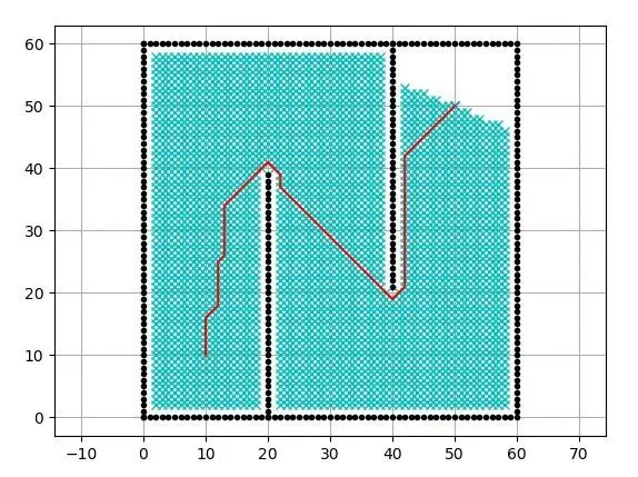
Grid-based shortest path planning using Dijkstra. Cyan points in the animation are visited nodes.
A*
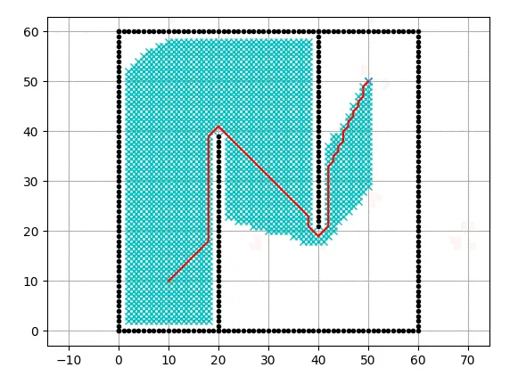
Grid-based shortest path planning using A*. Cyan points in the animation are visited nodes. The heuristic is the 2D Euclidean distance.
Potential Field
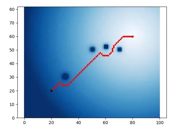
The blue heatmap shows potential values for each cell.
Further reading:
Motion planning: potential functions
https://www.cs.cmu.edu/~motionplanning/lecture/Chap4-Potential-Field_howie.pdf
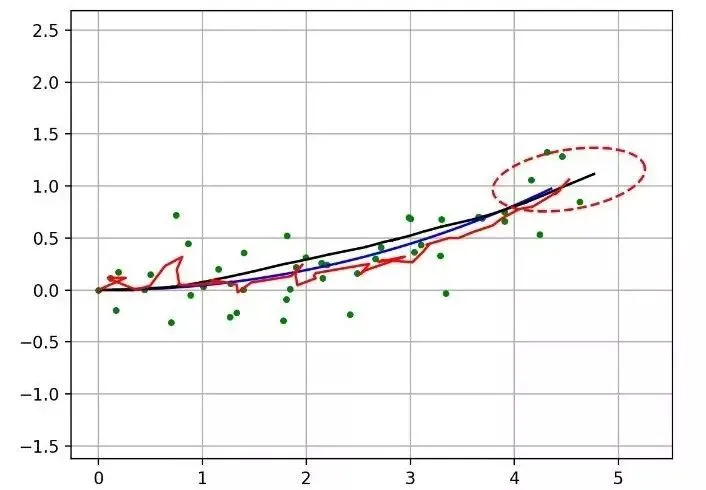
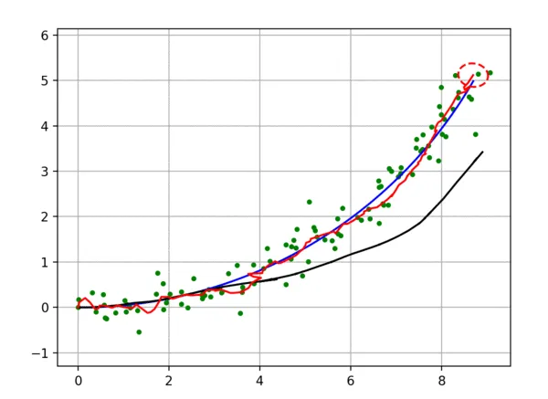
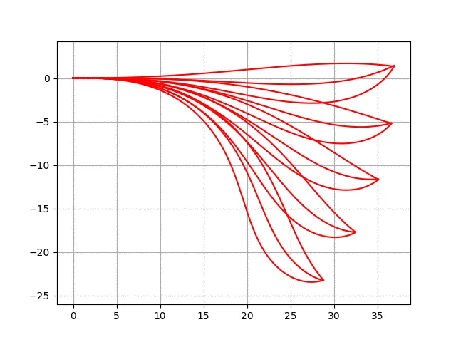
6.3 Model predictive path generation
Example of path optimization used for state lattice planning and lookup table generation.
Further reading:
Optimal path generation for wheeled robots over rough terrain
http://journals.sagepub.com/doi/pdf/10.1177/0278364906075328
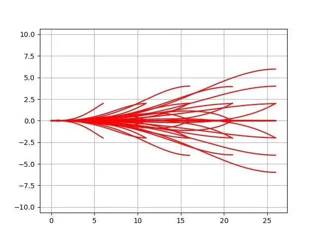
6.4 State lattice planning
State lattice planning example that uses model predictive path generation to handle boundary conditions.
Biased polar sampling example:
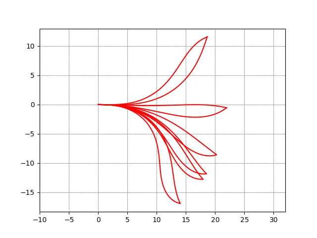
Lane sampling and other sampling strategies are included.
Further reading:
Optimal path generation for wheeled robots over rough terrain
http://journals.sagepub.com/doi/pdf/10.1177/0278364906075328
Feasible motion state space sampling for high-performance robot navigation in complex environments
http://www.frc.ri.cmu.edu/~alonzo/pubs/papers/JFR_08_SS_Sampling.pdf
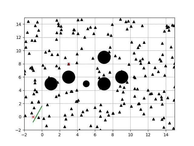
6.5 Probabilistic Roadmap (PRM)
PRM planning uses Dijkstra for graph search. Blue points are samples, cyan crosses are nodes visited by Dijkstra, and the red line is the final PRM path.
Further reading:
Probabilistic roadmap
https://en.wikipedia.org/wiki/Probabilistic_roadmap
6.6 Voronoi roadmap planning
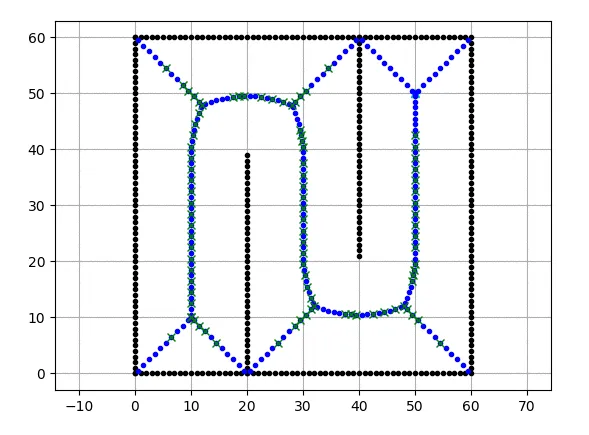
Voronoi roadmap planning using Dijkstra for graph search. Blue points are Voronoi nodes, cyan crosses are nodes visited by Dijkstra, and the red line is the final path.
Further reading:
Roadmap methods for motion planning
https://www.cs.cmu.edu/~motionplanning/lecture/Chap5-RoadMap-Methods_howie.pdf
6.7 Rapidly-Exploring Random Trees (RRT)
Basic RRT
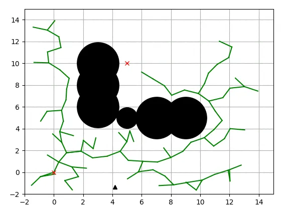
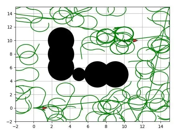
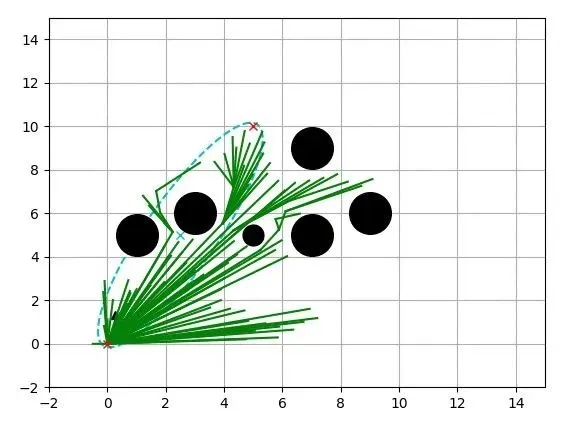
Basic RRT example. Black circles are obstacles, green lines are the search tree, and red crosses mark the start and goal.
RRT*
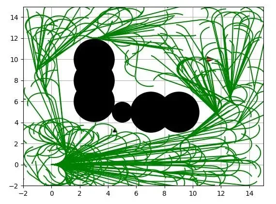
RRT* example. Black circles are obstacles, green lines are the search tree, and red crosses mark start and goal.
Further reading:
Incremental sampling-based algorithms for optimal motion planning
https://arxiv.org/abs/1005.0416
RRT with Dubins paths
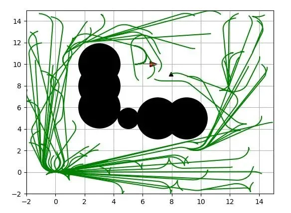
RRT and RRT* variants using Dubins paths for car-like robots.
RRT* with Reeds-Shepp paths
RRT* using Reeds-Shepp paths for vehicles that can go forward and reverse.
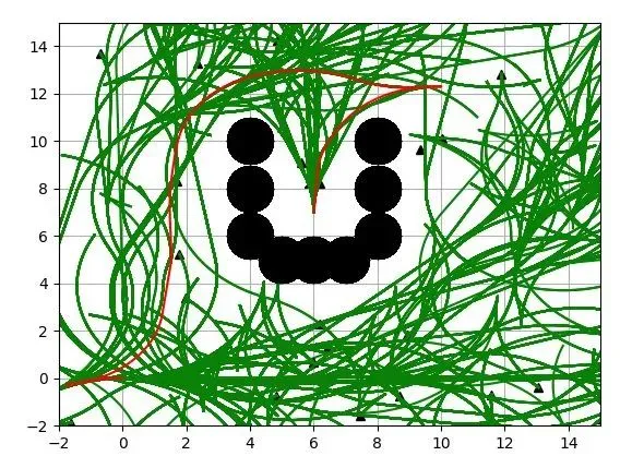
Informed RRT*
Informed RRT* example. The cyan ellipse shows the informed sampling domain.
Further reading:
Informed RRT*: Optimal sampling-based path planning via direct sampling of an admissible ellipsoidal subset
https://arxiv.org/pdf/1404.2334.pdf
Batch Informed RRT*
Batch Informed RRT* example.
Further reading:
Batch Informed Trees (BIT*): Heuristic search of implicit random geometric graphs for optimal sampling-based planning
https://arxiv.org/abs/1405.5848
Closed-loop RRT*
Closed-loop RRT* example using a pure-pursuit steering controller and PID speed control.
Further reading:
Motion planning with closed-loop prediction in complex environments
http://acl.mit.edu/papers/KuwataGNC08.pdf
LQR-RRT*
LQR-RRT* example using a double integrator motion model for local LQR planning.
Further reading:
LQR-RRT*: Optimal sampling-based motion planning using automatically derived extension heuristics
http://lis.csail.mit.edu/pubs/perez-icra12.pdf
6.8 Cubic spline planning
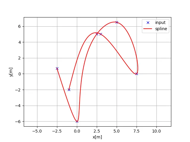
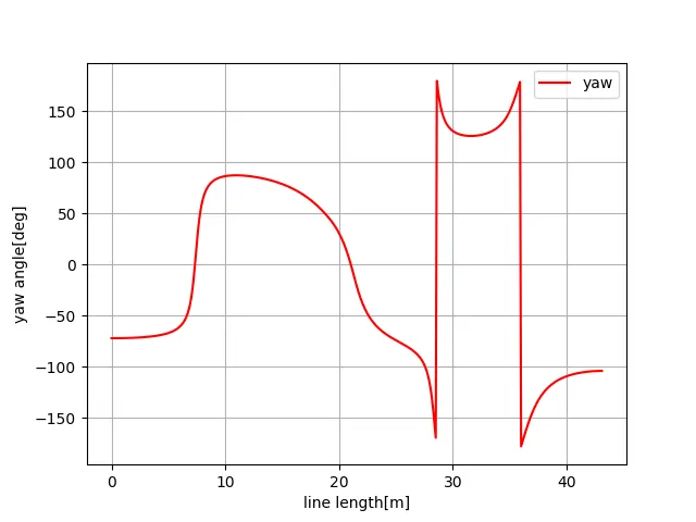
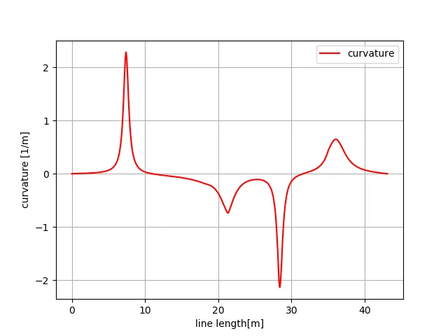
Example of cubic spline planning. Given x-y waypoints, generate a curvature-continuous path. Heading angles at each point can be computed analytically.
6.9 B-spline planning
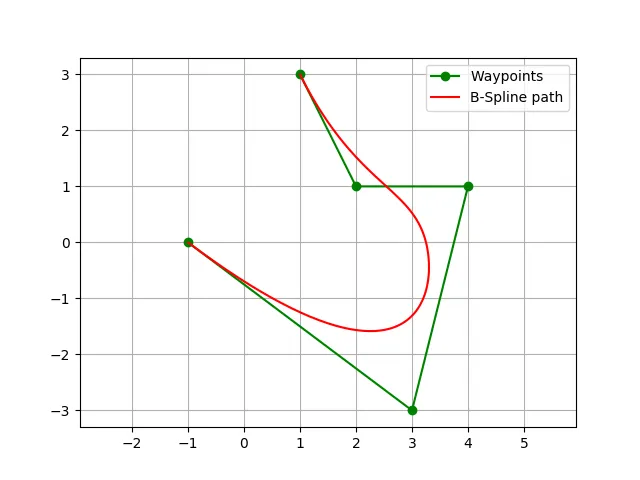
Example using B-splines to generate a smooth path from input waypoints. The first and last waypoints lie on the final path.
Further reading:
B-spline
https://en.wikipedia.org/wiki/B-spline
6.10 Eta^3 spline planning
Path planning using Eta^3 splines.
Further reading:
eta^3-Splines for the Smooth Path Generation of Wheeled Mobile Robots
https://ieeexplore.ieee.org/document/4339545/
6.11 Bezier path planning
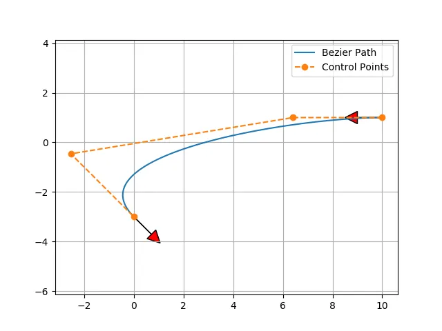
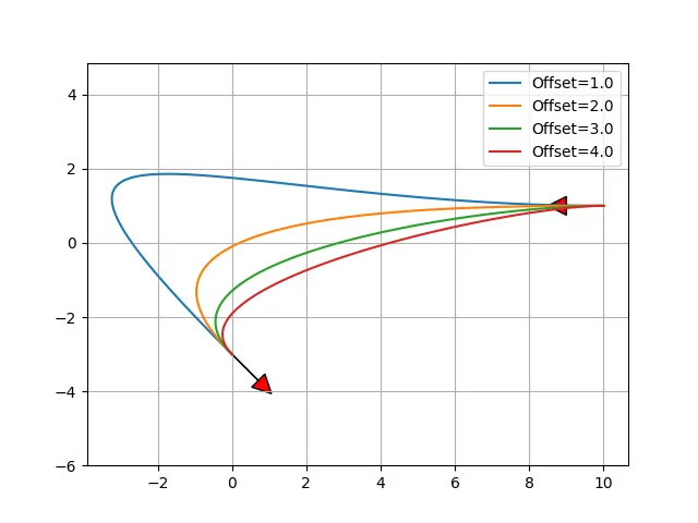
Example of Bezier path generation using four control points. Varying the start and end offsets produces different Bezier curves.
Further reading:
Generating curvature-continuous paths for autonomous vehicles using Bezier curves
http://citeseerx.ist.psu.edu/viewdoc/download?doi=10.1.1.294.6438&rep=rep1&type=pdf
6.12 Quintic polynomial planning
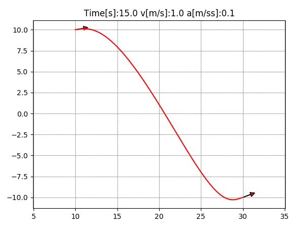
Compute 2D path, velocity, and acceleration using quintic polynomials.
Further reading:
Local path planning and motion control for AGV In-positioning
http://ieeexplore.ieee.org/document/637936/
6.13 Dubins path planning
Example implementation of Dubins path planning.
Further reading:
Dubins path
https://en.wikipedia.org/wiki/Dubins_path
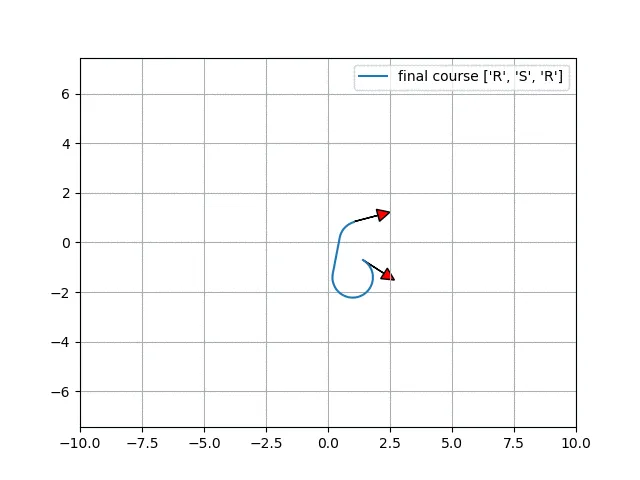
6.14 Reeds-Shepp path planning
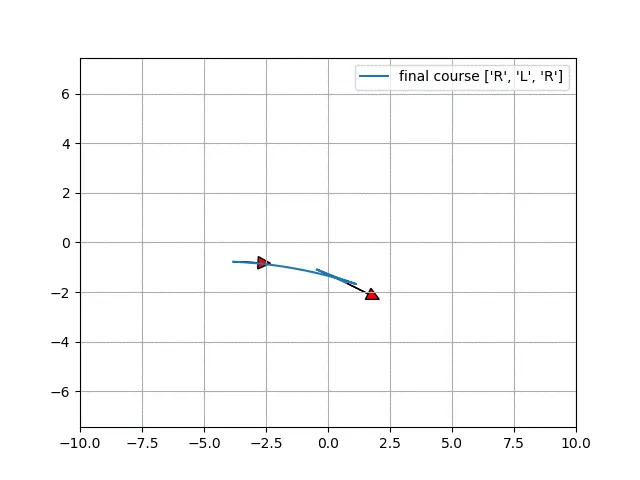
Example implementation of Reeds-Shepp path planning.
Further reading:
Reeds-Shepp curves
http://planning.cs.uiuc.edu/node822.html
6.15 LQR-based path planning
Example of LQR-based path planning for a double integrator model.
6.16 Optimal paths in the Frenet frame
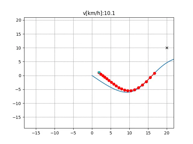
Generate optimal paths in the Frenet frame. The cyan line is the target path, black crosses are obstacles, and the red line is the predicted path.
Further reading:
Optimal Trajectory Generation for Dynamic Street Scenarios in a Frenet Frame
https://www.researchgate.net/profile/Moritz_Werling/publication/224156269_Optimal_Trajectory_Generation_for_Dynamic_Street_Scenarios_in_a_Frenet_Frame/links/54f749df0cf210398e9277af.pdf
Path tracking
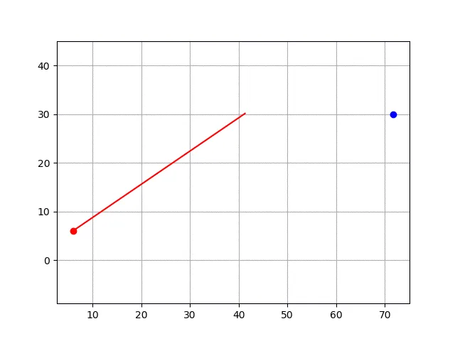
7.1 Pose control tracking
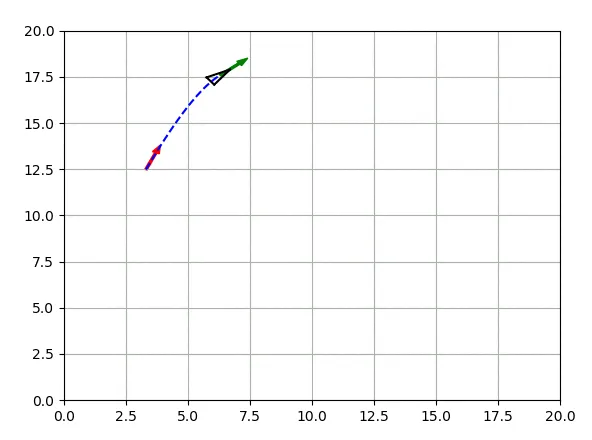
Pose control tracking simulation.
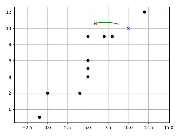
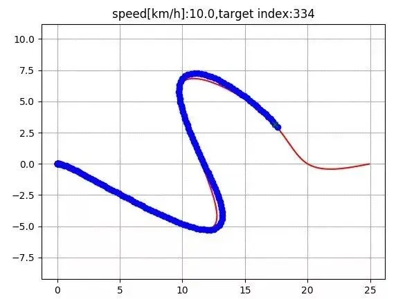
7.2 Pure pursuit tracking
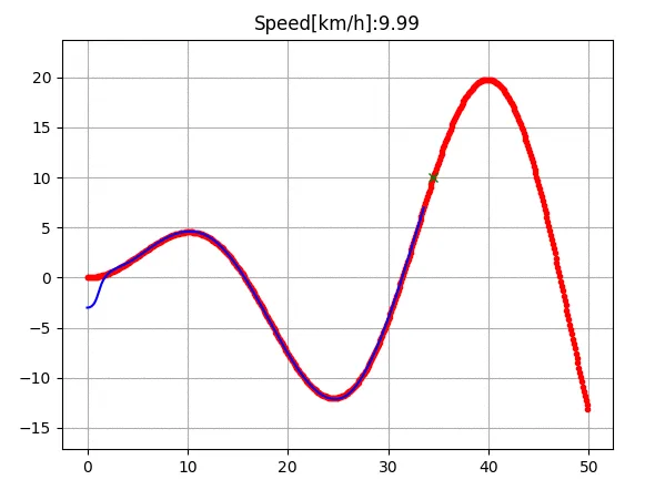
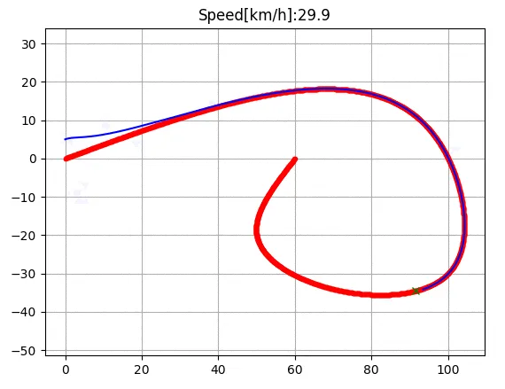
Pure pursuit steering and PID speed control tracking simulation. The red line is the target route, green crosses are pure pursuit lookahead points, and the blue line is the tracked route.
Further reading:
Survey of motion planning and control techniques for autonomous urban driving
https://arxiv.org/abs/1604.07446
7.3 Stanley control
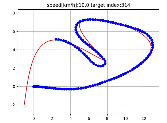
Stanley steering control with PID speed control tracking simulation.
Further reading:
Stanley: The robot that won the DARPA Grand Challenge
http://robots.stanford.edu/papers/thrun.stanley05.pdf
7.4 Rear-wheel feedback control
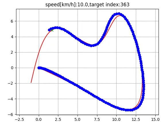
Rear-wheel feedback steering control with PID speed control tracking simulation.
7.5 LQR steering control
LQR steering control with PID speed control tracking simulation.
Further reading:
ApolloAuto/apollo open source autonomous driving platform
https://github.com/ApolloAuto/apollo
7.6 LQR steering and speed control
LQR steering and speed control tracking simulation.
7.7 Model predictive steering and speed control
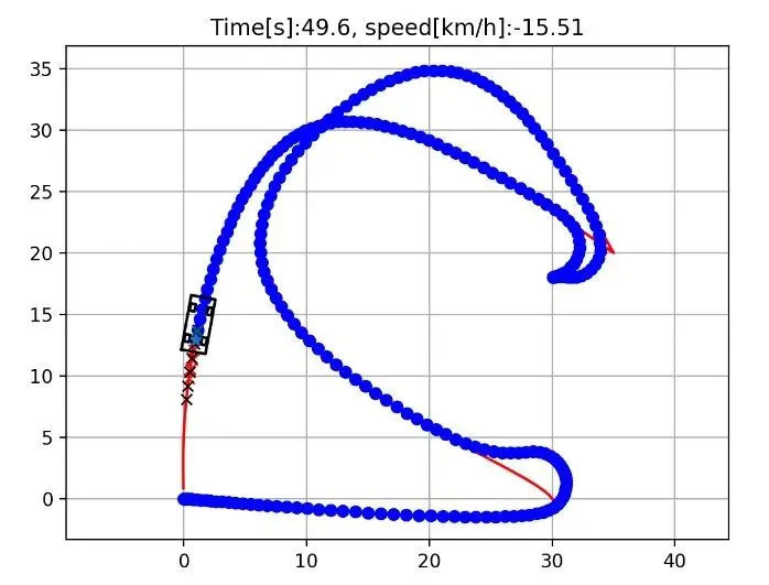
Iterative linear model predictive control example for steering and speed. This code uses cvxpy for optimization modeling.
Further reading:
Vehicle Dynamics and Control
http://www.springer.com/us/book/9781461414322