Overview
This article describes how to train neural networks to solve classification problems.
Neural network training process
The CIFAR network discussed in the first part of this series is composed of multiple neuron layers. Image data of 32 pixels x 32 pixels are presented to the network and propagated through the layers. The first step in a convolutional neural network (CNN) is to detect and analyze distinctive features and structures of the objects to be discriminated. This is done using filter matrices. After the designer models a neural network such as the CIFAR network, the filter matrices are initially unspecified, and at that stage the network cannot yet detect patterns or objects.
To enable detection, all parameters and elements of the filter matrices must be determined so as to maximize detection accuracy or minimize a loss function. This process is called neural network training. For common applications described in this series, networks are typically trained once during development and testing. After training, the networks can be used without further parameter adjustments. No additional training is required when the system is classifying familiar objects; training is needed only when the system must classify entirely new object types.
Training a network requires labeled training data and a separate set of similar data to test the network's accuracy. For example, in the CIFAR-10 dataset used in our example, the data are images belonging to ten object classes: airplane, automobile, bird, cat, deer, dog, frog, horse, ship, and truck. Preparing these labeled images is often the most complex part of developing an AI application. The training process discussed below is based on backpropagation. The network is repeatedly shown large numbers of images, each paired with a target label for the associated object class. On each presentation, the filter matrices are adjusted so that the network's output matches the target class. Once trained, the network can recognize objects that were not shown during training.
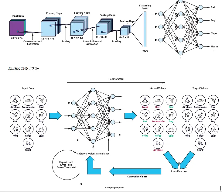
Figure 2. Training loop consisting of feedforward and backpropagation.
Overfitting and underfitting
A common question in neural network design is how complex the network should be: how many layers it should have, or how large the filter matrices should be. There is no simple answer. It is important to consider overfitting and underfitting. Overfitting results from a model that is too complex and has too many parameters. We can assess whether a predictive model fits the training data too well or too poorly by comparing training loss with test loss. If training loss is very low but loss increases dramatically when the network is presented with previously unseen test data, this strongly indicates the network has memorized the training set rather than generalized pattern recognition. This typically happens when the network has too many parameters or too many convolutional layers. In such cases the network size should be reduced.
Loss function and training algorithms
Learning proceeds in two steps. In the first step, an image is shown to the network and the neural network processes it to produce an output vector. The index of the maximum element of the output vector indicates the detected object class, for example "dog" in our example; during training this may not be correct. This step is called feedforward.
The difference between the target value and the actual output at the output layer is called the loss, and the corresponding function is called the loss function. All network elements and parameters are contained in the loss function. The goal of learning is to determine these parameters so as to minimize the loss function. This minimization is achieved by a process in which the deviation produced at the output (loss = target value minus actual value) is propagated backward through all components of the network until it reaches the input layer. This part of the learning process is called backpropagation.
Thus, training produces a loop that iteratively determines the filter matrix parameters. The feedforward and backpropagation steps are repeated until the loss falls below a predefined threshold.
Optimization algorithms, gradients, and gradient descent
To illustrate the training process, figure 3 shows a loss function depending on only two parameters x and y. The z axis corresponds to loss. The function here is schematic and used for illustration. Examining the three-dimensional surface, one can see global and local minima.
Many numerical optimization algorithms can be used to determine weights and biases. The simplest is gradient descent. Gradient descent is based on the idea of finding a path from a randomly chosen starting point on the loss surface toward a global minimum by taking iterative steps that use the gradient. The gradient is a vector operator that at each point on the loss function gives the direction of the steepest increase; its magnitude corresponds to the rate of change. On the surface in figure 3, a gradient vector will point toward a nearby minimum. Where the surface is flat, the gradient magnitude is low; where the surface is steep, the gradient magnitude is large.
Using gradient descent, one starts at an arbitrary point and iteratively follows the path of steepest descent toward a minimum. The optimizer computes the gradient at the current point and takes a small step in the direction of steepest negative gradient. At the new point, the gradient is recomputed and the process continues. This creates a path from the starting point to some point in the valley. The issue is that the starting point is randomly chosen. Depending on the starting point, the path may end at the global minimum or at a local minimum. In practice, networks optimize many thousands or millions of parameters, so the choice of starting point is effectively random. As a result, training time can be long, or the optimizer may converge to a local minimum rather than the global minimum, which reduces network accuracy.
Consequently, many optimization algorithms have been developed to address these issues. Alternatives include stochastic gradient descent, momentum, AdaGrad, RMSProp, and Adam, among others. The algorithm used in practice is chosen by the network developer, since each algorithm has specific advantages and disadvantages.
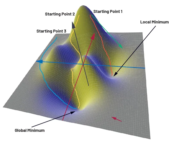
Figure 3. Different paths to reach a minimum using gradient descent.
Training data
As noted previously, the network is provided with images labeled with the correct object class (for example, automobile, ship, etc.) during training. In our example we used the CIFAR-10 dataset. In practice, AI applications often go beyond recognizing cats, dogs, and cars. For example, to develop an application that inspects the quality of screws in a manufacturing process, the network must be trained using images of both good and defective screws. Creating such a dataset can be labor-intensive and time-consuming and is often the most expensive step in developing an AI application. After compiling the dataset, it is split into training and test sets. Training data are used to train the network and test data are used at the end of development to verify the trained network's performance.
Conclusion
In the first part of this series, we described a convolutional neural network and examined its design and operation in detail. Now that the weights and biases required for the functions have been defined, we can assume the network operates as intended. In the final article of this series, we will test the network by converting it to hardware and using it to recognize cats. For this, we will use the MAX78000 AI microcontroller and a hardware-based CNN accelerator developed by ADI.