Overview
This article provides a concise introduction to visual perception for the autonomous driving industry, progressing from sensor comparisons and data collection/annotation to perception algorithms. It outlines key challenges and typical solutions for each module, and summarizes common framework design patterns for perception systems.
Perception objectives
Visual perception systems primarily use cameras as sensor inputs. After a series of computations and processing steps, the system estimates the surrounding environment to provide the fusion module with accurate and rich information. Typical outputs include object class, distance, velocity, orientation, and higher-level semantic information. Road traffic perception tasks can be grouped into three main areas:
- Dynamic object detection (vehicles, pedestrians, and micromobility)
- Static object recognition (traffic signs and traffic lights)
- Traversable area segmentation (road surface and lane lines)
Combining these tasks into a single neural network forward pass can increase throughput and reduce parameters. Increasing the backbone depth can further improve detection and segmentation accuracy. In practice, visual perception tasks are decomposed into object detection, image segmentation, object measurement, and image classification.
Sensor components
Forward narrow-angle camera
These modules typically have a field of view around 52° and are mounted near the center of the windshield. They are intended to perceive distant scenes in front of the vehicle, usually up to about 120 meters.
Surround wide-angle cameras
Wide-angle modules have a larger field of view, often around 100°, and are mounted around the vehicle to provide a 360° view. Their mounting scheme is similar to widely known production implementations such as Tesla. Wide-angle cameras exhibit noticeable distortion.
Surround fisheye cameras
Fisheye cameras provide fields of view exceeding 180° and are effective for short-range perception. They are commonly used for parking scenarios such as APA and AVP, and are mounted under side mirrors and near license plates to support image stitching, parking spot detection, and visualization.
Camera calibration
Calibration quality directly affects ranging accuracy. Calibration includes intrinsic calibration for lens distortion correction and extrinsic calibration to align coordinate systems across sensors, typically referencing the vehicle rear-axle center or another vehicle-level origin.
The classic calibration method uses a chessboard pattern. In production, per-vehicle tabletop calibration is impractical, so manufacturers construct calibration sites to perform calibration at vehicle delivery. Additionally, online calibration models exist to correct camera pose drift over time or after vehicle vibration, using detected features such as vanishing points or lane lines to update pitch in real time.
Data annotation
Real-world road scenarios present many unexpected situations, so large volumes of real vehicle data are required for training. High-quality annotation is critical. Perception systems require both object-level and pixel-level annotations.
Because detection and segmentation commonly use deep learning, which is data-driven, large amounts of labeled data are needed for iterative improvement. To increase annotation efficiency, semi-automatic annotation can be used: a neural network embedded in the annotation tool provides initial labels that are then corrected by annotators. New data and labels are periodically added for iterative retraining.
Functional modules
The visual perception pipeline is typically divided into several modules, including object detection and tracking, object measurement, traversable area estimation, lane detection, and static object detection.
Object detection and tracking
Detect and classify dynamic objects such as cars, trucks, e-bikes, bicycles, and pedestrians, and output class and 3D information. The module also performs frame-to-frame matching to stabilize detection boxes and predict object trajectories. Direct 3D regression from a network often lacks accuracy, so vehicles are sometimes detected as parts (front, body, rear, wheels) and assembled into a 3D bounding box.
Detection challenges include frequent occlusion, orientation estimation accuracy, diverse vehicle and pedestrian types that lead to false positives, and multi-object tracking issues such as ID switches. Visual-only perception degrades in adverse weather or low-light conditions, increasing missed detections. Fusing lidar data can substantially improve recall.
Detection approaches: provide 3D bounding boxes to recover orientation and height, and combine multi-object tracking for consistent IDs. Engineering constraints and geometry priors can augment deep learning outputs, for example fixed vehicle aspect ratios, bounded height for pedestrians, and physical continuity of vehicle distance. A practical pipeline uses a 3D (or 2.5D) detection model combined with backend multi-object tracking and monocular geometric ranging methods.
Object measurement
This module estimates longitudinal and lateral distance, and longitudinal and lateral velocity. Using detection and tracking outputs and ground priors such as the road plane, the system can compute distances and velocities from monocular images or regress object positions directly into a world coordinate system via neural networks.
Monocular measurement challenges:
- Estimating depth from a single camera without explicit depth measurements.
- Determining requirements, priors, and available maps.
- Specifying target accuracy and available computational resources.
- Assessing whether pattern recognition is robust enough for production verification standards.
Monocular measurement options:
- Use optical geometry (pinhole camera model) to relate world coordinates and image pixels, combined with camera intrinsics and extrinsics to compute distances to vehicles or obstacles.
- Directly regress a mapping from image pixels to distance using sampled images. This data-fitting approach lacks theoretical guarantees and is limited by fitting robustness.
Traversable area segmentation
Segment the vehicle drivable area by identifying vehicle footprints, curbs, visible obstacle boundaries, and unknown boundaries, and output a safe drivable region for the ego vehicle.
Challenges:
- Boundary shapes are complex in cluttered scenes, making generalization difficult. Unlike discrete detections (vehicle, pedestrian, traffic light), traversable space requires delineating any boundary that affects the vehicle, including unusual obstacles such as water barriers, cones, potholes, non-paved surfaces, green belts, patterned pavements, and complex intersections.
- Calibration drift: vehicle acceleration, bumps, and slopes change camera pitch, invalidating prior calibration and causing projection errors in distance and drivable boundary estimation.
- Edge point selection and post-processing: edges need filtering to remove noise and jitter. Incorrect projection of obstacle side boundaries can incorrectly label neighboring lanes as non-traversable.
Solutions:
- Perform camera calibration; if online calibration is not feasible, incorporate vehicle IMU data to adaptively adjust pitch-related parameters.
- Use a lightweight semantic segmentation network trained on broad scene coverage, label the required classes, sample edge points in polar coordinates, and apply filtering to smooth post-processed boundary points.
Lane detection
Detect lane types such as single/double-side lines, solid/dashed lines, double lines, color variants (white/yellow/blue), and special lane markings like merge lines and deceleration lines.
Challenges:
- Many line types and irregular surfaces make lane detection difficult. Standing water, worn markings, patched pavement, and shadows cause false or missed detections.
- Slopes and vehicle pitch changes can produce trapezoidal distortions in fitted lane lines.
- Curved lanes, distant lanes, and roundabout lanes complicate fitting and can cause flicker in detections.
Solutions:
- Traditional image-processing methods require undistorted images and perspective transform to a bird's-eye view, followed by feature operators or color-space extraction, histogram or sliding-window fitting. The limitation is poor adaptation across diverse scenes.
- Neural-network-based methods are similar to traversable area detection: choose a lightweight model and label appropriately. Lane fitting (cubic or quartic polynomials) is a challenge, so combine vehicle motion information (speed, acceleration, steering) and sensor data for dead reckoning to stabilize lane fits.
Static object detection
Detect static targets such as traffic lights and traffic signs.
Challenges:
- Traffic lights and signs are small objects occupying few pixels, making distant recognition difficult. Under strong backlight or glare, recognition is challenging even for humans. Correct traffic light detection is critical for intersection decisions when other vehicles are stopped at a zebra crossing.
- Sign class imbalance is common in collected datasets.
- Traffic light color is affected by illumination, making red/yellow differentiation hard in some lighting. At night, red lights can be similar to street or shop lighting, increasing false positives.
Solutions:
Perception-based recognition works but has limited robustness. Where the scene permits, auxiliary sources such as V2X and high-definition maps can provide redundancy. A practical priority order is: V2X > high-definition map > perception. When GPS is weak, perception results can be used for prediction, but V2X often covers many scenarios.
Common issues across modules
Although perception sub-tasks are implemented independently, they share upstream and downstream dependencies and common algorithmic problems.
Ground truth reference
Definition, calibration, and evaluation require reliable ground truth, not just visual inspection of detection outputs or frame rates. Use lidar or RTK data as ground truth to validate ranging accuracy under different conditions such as daytime, rain, or occlusion.
Resource consumption
Multiple networks and multiple cameras consume CPU and GPU resources. Consider how to allocate networks, whether forward passes can share convolutional layers, and whether threads or processes can coordinate modules efficiently. For multi-camera input, aim to maintain frame rate while handling multiple streams, including work on camera stream encoding and decoding.
Multi-camera fusion
Vehicles typically have four or more cameras. As an object moves from the rear to the front of the vehicle, it is observed by different cameras. The object ID should remain consistent across camera views, and distance estimates should not jump significantly when switching between cameras.
Scene definition
Define datasets and scenes clearly for each perception module to enable targeted algorithm validation. For dynamic object detection, separate stationary-vehicle scenarios from moving-vehicle scenarios. For traffic lights, subdivide into scenarios like left-turn lights, straight-through lights, and U-turn lights. Validate on both public and proprietary datasets.
Module architecture
Open-source perception frameworks such as Apollo and Autoware influence many research groups and smaller companies. A typical camera-based perception pipeline follows this flow:
Camera input → image preprocessing → neural network → multiple branches (traffic light recognition, lane detection, 2D detection to 3D conversion) → post-processing → output (object class, distance, velocity, orientation).
Input frames are processed per-frame for detection, classification, and segmentation, then multi-frame information is used for multi-object tracking and final outputs. The core stages are neural network algorithms whose accuracy, speed, and hardware efficiency must be balanced. Common difficulties include false positives and misses in object detection, high-order curve fitting for lanes, small-object detection for traffic lights at long distance, and high precision requirements for traversable boundary points.