Overview
Bandwidth, sampling rate, and memory depth are the three key specifications of a digital oscilloscope. Compared with bandwidth, sampling rate and memory depth are often overlooked during instrument selection, evaluation, and testing. This article explains sampling rate and memory depth theory and common application impacts to help engineers understand their importance, trade-offs when choosing an oscilloscope, and correct usage practices.
Before introducing sampling and memory concepts, briefly recall the operating principle of a digital storage oscilloscope.
The input voltage signal passes through the coupling circuit to the front-end amplifier, which increases sensitivity and dynamic range. The amplifier output is sampled by the sample-and-hold circuit and digitized by an A/D converter. After A/D conversion, the signal is stored as digital data in memory. A microprocessor processes the stored digital waveform and displays it on the screen. This is the basic operation of a digital storage oscilloscope.
Sampling and Sampling Rate
Computers process discrete digital signals. The primary challenge when an analog voltage signal enters an oscilloscope is converting the continuous signal to discrete samples. The process of converting a continuous signal to discrete samples is called sampling. A continuous signal must be sampled and quantized before a computer can process it. Sampling measures the waveform voltage at equal time intervals and converts that voltage into a digital code. The smaller the time interval between samples, the closer the reconstructed waveform matches the original signal. Sampling rate is the frequency of sampling. For example, a sampling rate of 10 GSa/s means a sample is taken every 100 ps.
According to the Nyquist sampling theorem, when sampling a band-limited signal with maximum frequency component fmax, the sampling frequency SF must be greater than twice fmax to ensure complete reconstruction of the original signal from samples. If sampling falls below the Nyquist rate, aliasing occurs. For a sine wave, each cycle needs at least two samples to approximately reconstruct the waveform. Aliasing can produce deceptive waveforms and incorrect frequency measurements.
For higher-frequency signals, always monitor the oscilloscope sampling rate to avoid aliasing. It is recommended to set the oscilloscope sampling rate before measurements to prevent undersampling.
From Nyquist, a maximum real-time sampling rate of 10 GS/s can theoretically capture frequency components up to 5 GHz, which is the theoretical digital bandwidth (half the sampling rate). This theoretical digital bandwidth differs from the oscilloscope's analog bandwidth commonly specified on instrument panels.
In practical digital storage oscilloscopes, the required sampling rate for a given bandwidth depends on the sampling mode used.
Sampling Modes
Before A/D conversion, input signals must be sampled. Sampling techniques fall into two broad categories: real-time sampling and equivalent-time sampling.
Real-time sampling captures non-repetitive or single-shot signals using fixed time intervals. After triggering, the oscilloscope samples continuously and reconstructs the waveform from those samples.
Equivalent-time sampling samples different cycles of a repetitive waveform and stitches sample points together to recreate the waveform. Equivalent-time sampling requires repeated triggers and includes sequential sampling and random interleaved sampling. It requires that the waveform be repetitive and that triggering be stable.
In real-time mode, the oscilloscope bandwidth depends on the A/D converter maximum sampling rate and the interpolation algorithm used. Real-time bandwidth, also called effective storage bandwidth, depends on the A/D and interpolation algorithm.
To summarize: oscilloscope bandwidth has two concepts. Analog bandwidth is the commonly specified panel bandwidth. Storage bandwidth is the theoretical digital bandwidth derived from sampling theory. Effective storage bandwidth BWa can be defined as:
BWa = maximum sampling rate / k
For single-shot signals, maximum sampling rate refers to the highest real-time sampling rate of the A/D converter. For repetitive signals, it refers to the highest equivalent sampling rate. The factor k depends on the interpolation algorithm. Common interpolation methods are linear interpolation and sinx/x interpolation. k is about 10 for linear interpolation and about 2.5 for sinx/x interpolation, although k = 2.5 only applies when reproducing sine waves; for pulses k = 4 is often used. For example, a 1 GS/s oscilloscope with k = 4 has an effective storage bandwidth of 250 MHz.
In practice, using sinx/x interpolation requires a sampling rate at least 2.5 times the highest frequency component for accurate reconstruction. Using linear interpolation requires a sampling rate at least 10 times the highest component. This explains why maximum sampling rates for real-time sampling are often four times or more the rated analog bandwidth.
Vertical Resolution
Vertical resolution is closely related to the A/D converter and determines the smallest voltage increment the oscilloscope can resolve. It is usually given by the number of A/D bits n. Many oscilloscopes use 8-bit A/D converters, so the quantization step is 1/256, or about 0.391%. This affects amplitude measurements. For example, if the vertical scale is 1 V/div and the scope has 8 vertical divisions, the smallest resolvable change is approximately 8 V × 0.391% = 31.25 mV. Changes smaller than this cannot be resolved at that scale. To improve amplitude accuracy, scale the waveform to fill the screen and fully use the available resolution.
Note that an oscilloscope is not a precision metrology instrument. It is a diagnostic tool that helps engineers visualize circuit behavior.
Storage and Memory Depth
After A/D digitization, the binary waveform samples are written to the oscilloscope's high-speed CMOS memory. The memory capacity, or memory depth, is important. While the oscilloscope's maximum memory depth is fixed, the actual record length used in a test can be adjusted.
For a given memory depth, higher sampling rates shorten the available acquisition time; they are inversely related. Sampling rate corresponds to write speed and acquisition time corresponds to record length. The relationship is:
Memory depth = sampling rate × acquisition time
Because an oscilloscope display window is typically divided into 10 horizontal divisions, acquisition time = time base × 10.
Increasing memory depth allows capturing longer time spans at higher sampling rates. If memory depth is limited, sampling rate must be reduced to capture long records, which degrades waveform fidelity. Increasing memory depth enables higher sampling rates and undistorted waveforms.
Figure 1 shows how memory depth affects actual sampling rate for a given time base. For example, with a 10 us/div time base, the total window is 100 us. With 1 Mpoints memory depth, the actual sampling rate is 1 M / 100 us = 10 GS/s. If memory depth is only 250 kpoints, the actual sampling rate drops to 2.5 GS/s.
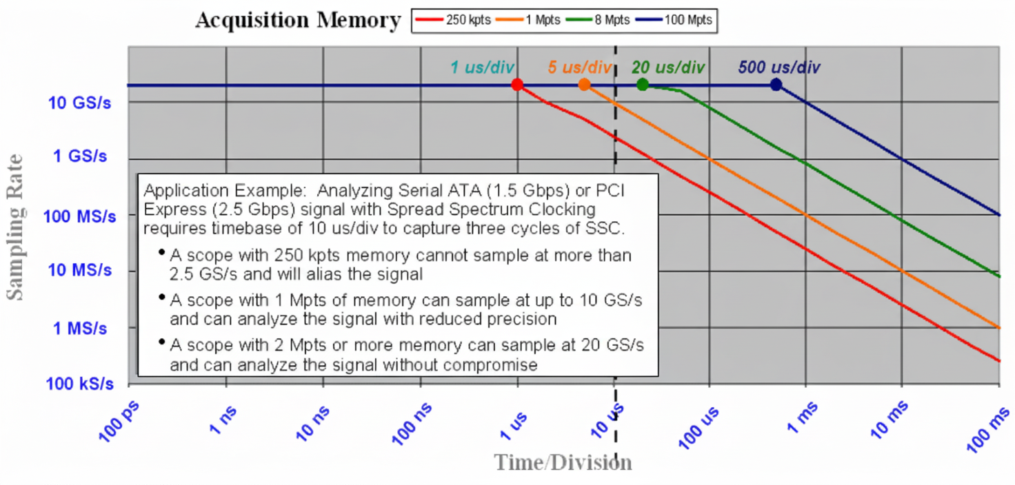
Figure 1 Memory depth determines actual sampling rate
In short, memory depth determines the oscilloscope's ability to analyze high- and low-frequency phenomena simultaneously, including high-frequency noise on low-speed signals and low-frequency modulation on high-speed signals.
Importance of Long Records in Power Measurements
Power electronics operate at relatively low frequencies (often below 1 MHz). Although a 500 MHz bandwidth oscilloscope is sufficient for hundreds of kHz switching frequencies in theory, sampling rate and memory depth choices are critical in practice. For example, switching power supplies often switch at 200 kHz or faster and exhibit line-frequency modulation. Engineers may need to capture quarter-cycle, half-cycle, or multiple cycles of line-frequency components. If switching edges have 100 ns rise time and at least five samples on the edge are required, then the sampling rate needs to be at least 5 / 100 ns = 50 MS/s, so sample interval < 20 ns. To capture one 50 Hz line cycle (20 ms), the required memory depth per channel is 20 ms / 20 ns = 1 Mpoints. Capturing soft-start sequences during power-up may require even longer records and higher memory depth.
Using an oscilloscope with only 10 kpoints per channel for such power tests is insufficient. Adequate memory depth is essential for correct power measurements.
Effect of Memory Depth on FFT Results
Fast Fourier Transform (FFT) on an oscilloscope yields the signal spectrum for frequency-domain analysis, such as power harmonics or noise sources. The total acquisition memory determines the Nyquist frequency and the frequency resolution △f. Frequency resolution is △f = 1 / acquisition time. For example, to achieve 10 kHz resolution, acquisition time must be at least 1 / 10 kHz = 100 ms. For an oscilloscope with 100 kB of memory, the highest analyzable frequency is:
△f × N/2 = 10 kHz × 100 k / 2 = 500 MHz
Longer record lengths improve FFT results by increasing frequency resolution and improving signal-to-noise ratio. Some detailed information may only be visible at very large memory depths, such as 20 Mpoints, as shown in the next figures.
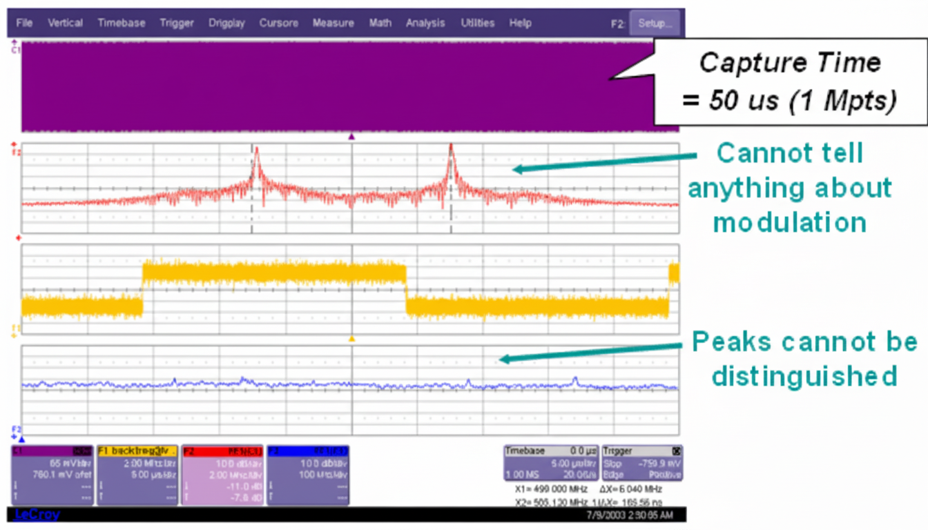
Figure 2 FFT with 1 Mpoints cannot reveal modulation information
Note that long-record FFT analysis requires strong data processing capability, which exceeds some instruments' limits. Different oscilloscope models vary in maximum FFT point capability.
High-speed Serial Signal Analysis and Real Long Records
Jitter analysis and eye diagram testing are essential for high-speed serial link analysis. For jitter testing, high acquisition memory length is a key specification. Memory depth determines sample count per jitter test and the lowest jitter frequencies that can be analyzed. All jitter has frequency components from DC to high frequencies. The inverse of the single-shot acquisition window indicates the jitter frequency range that can be observed. For example, capturing a 2.5 Gbps signal with a 20 GS/s sampling rate and 1 Mpoints memory yields a 50 μs acquisition window, allowing detection of jitter periods down to 20 kHz. A 20 GS/s sampler with 100 Mpoints memory can detect jitter down to 200 Hz.
Some oscilloscope architectures implement many high-speed ADCs and on-chip memory inside a single SoC. That limits on-chip high-speed memory (often less than 2 Mpoints at very high sample rates) and restricts low-frequency jitter analysis. External low-speed memory can be used to extend record length but typically cannot operate at the highest sampling rates, limiting meaningful jitter analysis at full speed. For example, at 40 GS/s with 512 kpoints memory, the single acquisition is only 12.5 μs, limiting jitter measurement to frequencies above 80 kHz, which may be insufficient for many applications.
Eye diagram analysis also benefits from large real-time memory. Some instruments can perform real-time, dynamic eye measurements on millions of unit intervals (UI), while others can only process small UI subsets or rely on offline software with lower efficiency. For example, for a PCIe Gen2 eye test at 5 Gb/s, 1 million UI corresponds to 200 μs. At 40 GS/s this requires about 8 Mpoints. Insufficient memory or processing capability may prevent capturing and analyzing such a dataset in a single, reliable measurement.
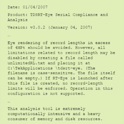
Figure 3 Manufacturer internal note on eye diagram processing limits
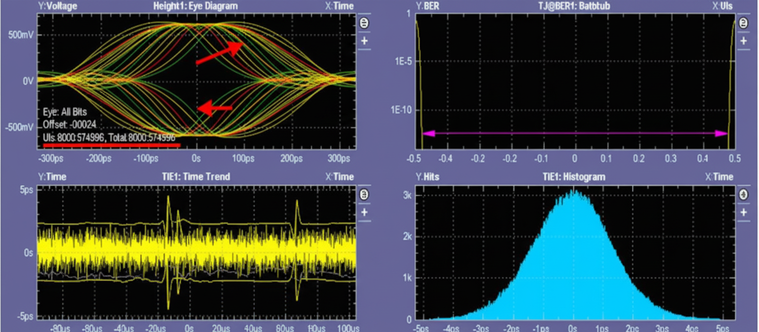
Figure 4 Example test: eye diagram from a subset of captured UI