Image-based vision processing typically requires camera calibration before experiments to obtain the relevant parameters. For convenience, three commonly used camera calibration methods are summarized below.
Intrinsic Camera Calibration
Step 1: Place a checkerboard pattern in front of the camera and rotate it around all axes. Keep rotation angles within 45 degrees. Capture images from different orientations for later processing.
Step 2: Open Matlab and launch the Camera Calibration app. Import the captured checkerboard images. Ensure you have 20–30 correctly imported images. Measure the real size of each checkerboard square and enter that value into Matlab.
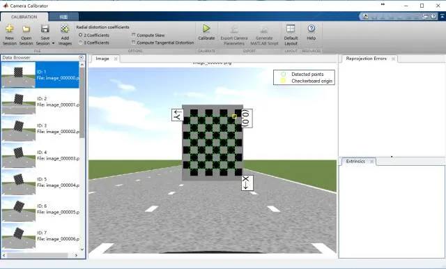
Step 3: Verify that checkerboard corners are detected correctly, then click the Calibrate button and observe the reprojection error. If some images have large reprojection errors, remove them and recalibrate until the results are satisfactory.
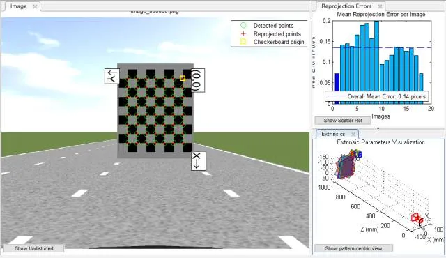
Step 4: Select the Export Camera Parameters button to export the computed parameters. For higher accuracy, consider modeling lens distortion or use stereo calibration methods.
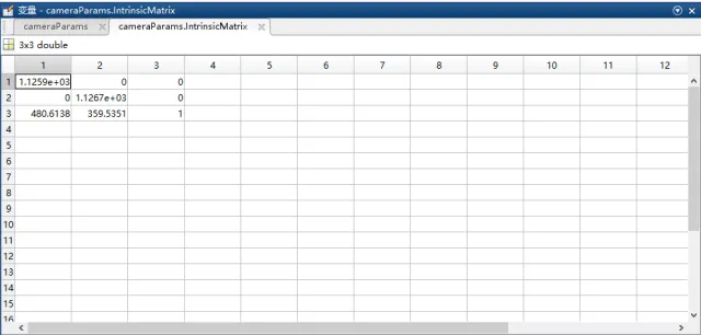
The example intrinsic matrix shows fx=1.1259e+03, fy=1.1267e+03, u=480.6138, v=359.5351.
Notes:
- The checkerboard should occupy a sufficiently large area in the image so that corners are detected clearly.
- The intrinsic matrix obtained from Matlab is the transpose of the intrinsic matrix conventionally calculated in some workflows.
- If performing radar-camera joint calibration, some calibration steps need to be adjusted.
Inverse Perspective Mapping (IPM) Calibration
Step 1: Draw a vertical line along the image center. From the vehicle's front center, place a straight measuring reference along the image centerline. A typical distance is around 15 m.
Step 2: On a flat surface within the camera field of view, select a rectangle whose longitudinal axis aligns with the image centerline. Mark the four corners of the rectangle so they are clearly visible in the camera image.
Step 3: Start the calibration program and enter the X-axis offset a, Y-axis offset b, rectangle width w, rectangle height h, and a scale factor k. Example initial values are: 1280, 445, 360, 600, 4.5. Then select the rectangle corners in order: top-left, top-right, bottom-left, bottom-right, aligning the program's guide lines with the rectangle edges in the image. The calibration returns the homography matrix H for inverse perspective mapping. Verify H in practical tests to ensure reasonable results. Ensure the image shows the current lane and adjacent lanes, and that parallel lines remain parallel after mapping.
Notes:
- The calibrated IPM image region and the test IPM image region should have the same dimensions.
- The two rectangle corners closer to the camera should be placed as near to the vehicle as possible; placing them near the vehicle blind spot tends to produce more accurate H.
- Coordinate conventions: the world coordinate system is the 2D plane of the road surface where the vehicle is located. X is lateral, Y is longitudinal. The image coordinate system has its origin at the top-left corner; X increases to the right and Y increases downward. Thus the four rectangle corner coordinates are (a/k, b/k), ((a+w)/k, b/k), (a/k, (b+h)/k), ((a+w)/k, (b+h)/k). Parameters a, b, h, k are in centimeters. When a is positive, the IPM image shifts right; when b is positive, the IPM image shifts down. Increasing lateral offset widens the lateral field of view in the bird's-eye image; increasing longitudinal offset extends the forward field.
Monocular Distance Calibration
(1) Longitudinal Distance Calibration
Required items: checkboard calibration for intrinsic parameters and a measuring reference for ground distances.
The geometric model relates image pixel coordinates to world distances based on the camera imaging geometry and the camera-to-ground relationship, as shown below.
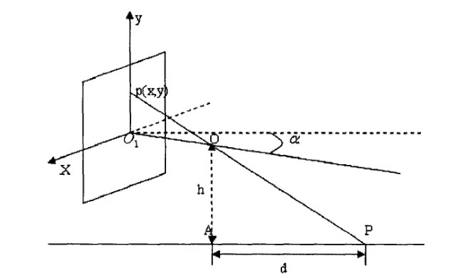
From the geometric model, derive the relation between image physical coordinates and world distance.
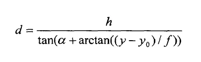
Using the conversion between image physical coordinates and pixel coordinates:
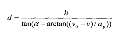
In these formulas, ay denotes the effective focal length along the y direction, alpha denotes the camera pitch angle, v0 denotes the principal point y-coordinate, and v is the pixel row coordinate. Alpha can be solved from calibration and measurements.
Experimental steps:
- Use checkerboard calibration to obtain fv and v0, and measure the camera height h above ground.
- Draw a vertical line along the image center. Place a straight measuring reference along that centerline in front of the vehicle for about 60 m, and measure the distance from the camera to the reference origin.
- Select 15 markers from far to near and record each marker's true distance to the camera. Establish one-to-one correspondences between pixel positions and true distances. Solve for the camera pitch angle using the geometric relations above, then compute longitudinal distances to objects ahead.
(2) Lateral Distance Calibration
Calibration principle:
For a monocular camera, all lines parallel to the camera optical axis converge to a single vanishing point L. Any point on the line connecting the point of interest and the vanishing point has the same distance to the optical axis in the image.
Establish a pixel-based coordinate system with the image top-left as the origin. Represent the test point in pixel coordinates, compute the angle between the line from the test point to the vanishing point and the optical axis, and match that angle to the actual lateral distance from the optical axis. Fit data to derive the mapping from image angle to lateral distance.
Experimental steps:
- Park the vehicle in the lane center with lane markings parallel to the vehicle longitudinal axis. Select two points on a lane marking in the image and one point on the image centerline to compute the vanishing point coordinates.
- At a fixed distance ahead (commonly 15 m), place 10 obstacles laterally along one side of the vehicle centerline. In the image, pick the obstacles from left to right and compute the angle between each obstacle-to-vanishing-point line and the optical axis. Record each obstacle's true lateral distance to the vehicle center. Establish the correspondence between angle and true distance, and perform curve fitting in Matlab. During testing, measure the pixel position, compute the angle, and use the fitted curve to estimate the lateral distance from the vehicle center.