1. Introduction
Phase noise is one of the basic metrics of an oscillator. Experienced engineers can learn a great deal about oscillator quality and its suitability for an application by inspecting a phase noise plot. RF engineers focus on phase noise levels at specific carrier offset frequencies to ensure the required modulation schemes are supported. Designers of high-speed serial links such as 40GbE apply band-pass filters to the reference clock phase noise, integrate the result and convert it to phase jitter to predict system bit error rate.
This application note first provides a brief theoretical overview of phase noise and phase noise measurement methods, then focuses on practical measurement advice such as how to connect the signal under test to the instrument, how to configure a phase noise analyzer, and how to select an appropriate analyzer. All measurements in this document were performed using the Keysight E5052B phase noise analyzer, a commonly used instrument for phase noise measurements.
2. What Is Phase Noise
Phase noise is the frequency-domain representation of short-term phase instability of a signal. It is commonly described as single-sideband (SSB) phase noise and denoted as L(f). The classic definition of phase noise is the ratio of the power spectral density measured at a carrier offset frequency to the total signal power. For practical use, this definition is slightly modified so that the power spectral density measured at the carrier offset frequency is referenced to the carrier power rather than the total integrated signal power (see Figure 2-1).
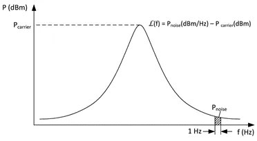
Figure 2-1: Classic phase noise definition
When measuring phase noise with a spectrum analyzer, the classic definition is convenient but it combines amplitude and phase noise effects. It also has limitations for signals with high phase noise. The classic definition typically applies when peak-to-peak phase deviation is much less than 1 radian. It can never exceed 0 dB because noise power in the signal cannot exceed the signal's total power.
More recently, phase noise has been redefined as half the power spectral density of phase fluctuations, L(f) = S_phi(f)/2. An ideal sine wave can be written as f(t) = A sin(omega t + phi). A sine wave with phase noise is f(t) = A sin(omega t + phi(t)), where phi(t) is the phase noise. S_phi(f) is the power spectral density of phi(t). Defined this way, phase noise is separated from amplitude noise and can exceed 0 dB, which indicates phase variations greater than 1 radian.
3. Phase Noise Measurement Methods
There are two widely used phase noise measurement methods. The first uses a spectrum analyzer to measure the power spectrum and the classic phase noise definition. The signal spectrum is measured with a given resolution bandwidth and the phase noise is then calculated as shown in Figure 2-1.
The second method is compatible with the modern phase noise definition using S_phi(f) and employs phase detection techniques. The basic principle is to compare the device under test (DUT) to a reference signal using a phase detector. The phase detector output is proportional to the phase difference between its inputs (see Figure 3-1).
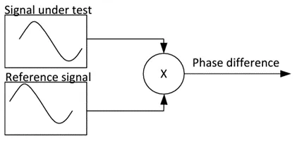
Figure 3-1: Phase detector method for phase noise measurement
There are many variants of the phase detector method. The Keysight E5052B implements two variants of this approach, labeled in the instrument as "normal" and "wide."
Normal mode is a PLL-based method that locks a reference oscillator to the DUT using a PLL. This keeps the reference and source signals at a 90° phase difference at the phase detector inputs. The phase detector output is sampled with an ADC and S_phi(f) is computed using a fast Fourier transform (FFT).
In wide measurement mode, the E5052B uses a heterodyne (digital) discriminator method. An analog mixer downconverts the DUT to an intermediate frequency (IF), which is then sampled by an ADC. The phase detector is implemented in the DSP by comparing the signal to a delayed version of itself. The phase detector output is filtered with a digital low-pass filter to separate the phase difference component from high-frequency components. The resulting time-domain digital signal that represents phase noise is then processed in the DSP using FFT and normalization.
Normal mode is suitable for stable clock sources. It provides optimal sensitivity and wide offset coverage. For signals with high near-carrier phase noise, wide mode is recommended. Cross-correlation can be used to improve the sensitivity of the heterodyne (digital) discriminator method, especially at close offsets.
4. Connecting the Signal to the Phase Noise Analyzer
4.1 Signal Level and Thermal Noise
Thermal noise is electronic noise generated by the thermal motion of charge carriers in conductors. It is expressed as the average noise power per hertz of bandwidth at a given temperature. Higher resistor temperature increases the kinetic energy of charge carriers, producing more noise. Thermal noise is essentially broadband with an approximately flat spectrum.
Thermal noise can limit the noise floor of phase noise measurements for weak signals. The thermal noise floor at room temperature is -174 dBm/Hz. The phase noise portion of thermal noise is 3 dB lower, yielding -177 dBm/Hz at room temperature. The theoretical phase noise measurement floor is the difference between the carrier signal power and the phase-noise portion of the thermal noise. Table 4-1 shows the theoretical phase noise measurement floor as a function of input signal power.
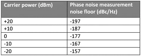
Table 4-1: Theoretical phase noise measurement floor as a function of signal power
4.2 Active Amplifiers and Probes
An active amplifier may be required to route the DUT signal to a phase noise analyzer when the signal is too weak to drive the instrument's 50 ohm input directly. A typical example is the clipped-sine output often seen in precision TCXOs and OCXOs. The impedance of a clipped-sine driver is relatively high and cannot directly drive a 50 ohm load. Another example is measuring phase noise on a customer board without loading the circuit.
Any active amplifier has its own noise figure and will add noise to the source signal as the signal passes through the amplifier. As a result, the signal-to-noise ratio at the amplifier output is reduced compared to the input. If amplification or buffering is necessary before connecting the DUT to the phase noise analyzer, the amplifier's noise figure must be considered to ensure the amplifier-added noise is negligible.
Active probes provide a convenient way to access signals on a system or evaluation board. They add minimal parasitic loading and come with accessories to connect to traces, pins, probe points, or other features. Active probes are primarily designed for precise waveform measurements of high-bandwidth signals. Two main issues arise when using active probes for phase noise measurements:
1. Active probes have high bandwidth and introduce substantial wideband noise to the signal.
2. To achieve high bandwidth, amplifiers inside active probes often attenuate the signal before presenting it to the analyzer. This reduces signal power at the analyzer input and raises the measurement noise floor due to thermal noise.
Active probes are not recommended for phase noise measurements.
4.3 Oscillator Output Signal Types
Oscillators can present different output signal types. The two main categories are single-ended and differential outputs. Single-ended signals carry the clock on one line relative to common ground. Differential signals use two lines carrying the clock 180° out of phase with each other.
The following gives guidance for connecting the most common signal types to a phase noise analyzer.
4.3.1 Single-ended LVCMOS
LVCMOS is a single-ended output type, usually swinging between 0 V and VDD. Output impedance is typically between 20 ohm and 40 ohm. LVCMOS outputs can often be connected directly to a 50 ohm analyzer input, but observe the following:
1. Use a 50 ohm coaxial cable for the connection, preferably short (<= 3 ft) to minimize insertion loss and signal attenuation.
2. The analyzer input has a 50 ohm termination, and connecting a 50 ohm load to the oscillator will draw significant current from the output driver. This additional power dissipation slightly increases the internal chip temperature. Another effect of higher driver current is an increase in spurious harmonic components in the phase noise if the driver influences other modules in the oscillator circuit. These spurious levels may be higher than under normal load conditions.
4.3.2 Single-ended Clipped Sine
Clipped-sine outputs are single-ended with slow edges and reduced signal amplitude; they are common in precision TCXOs and OCXOs. These outputs have relatively high source impedance (kilo-ohm range). Directly connecting a clipped-sine output to a 50 ohm analyzer input yields low signal power and thermal noise will significantly limit the measurement floor. For example, a clipped-sine source with 1 kΩ source impedance and 1 Vpp provides approximately -20 dBm to a 50 ohm instrument input, resulting in a theoretical measurement floor of -157 dBc/Hz, which is not acceptable for a clock that should reach -170 dBc/Hz at a 5 MHz offset.
To avoid this, the signal power must be raised to an acceptable level. One option is a low-noise RF amplifier such as the Mini-Circuits ZX60-3018G-S+, which has SMA input and output and can be easily inserted into the measurement setup.
4.3.3 Differential Outputs
Common differential output types include LVPECL and LVDS. Less common types such as HCSL are still used in some applications. Differential outputs offer benefits including common-mode noise rejection, immunity to coupled noise, strong power-supply noise rejection, and good high-frequency performance.
Phase noise analyzers usually have single-ended inputs, but differential outputs have two outputs. The simplest approach to connect a differential output to a single-ended 50 ohm instrument is to connect one differential output directly to the instrument and terminate the other output to ground with 50 ohm. The disadvantages are that common-mode noise is not cancelled, which can raise the noise floor, and half the signal power is lost. As noted earlier, weaker signal power increases the influence of thermal noise.
A better solution is a balun (balanced-to-unbalanced transformer) to convert the differential signal to single-ended before connecting to the phase noise analyzer. A balun is a high-frequency transformer where the differential signal is applied to the primary winding and the single-ended signal is taken from the secondary winding. Figure 4-2 illustrates the phase noise of a SiT9365 differential oscillator measured in single-ended mode (one output connected to the analyzer) and using a JTX-2-10T RF transformer as a balun. The single-ended measurement exhibits a higher noise floor.
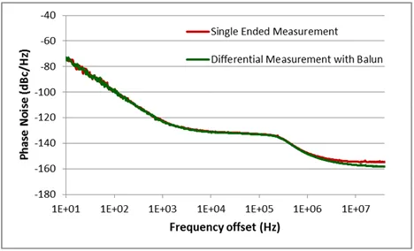
Figure 4-2: Phase noise of the SiT9365 156.25 MHz differential oscillator measured in single-ended and differential modes
5. Setting Up the Phase Noise Analyzer
5.1 Auto Setup
Most phase noise analyzers offer an auto-setup feature intended to select optimal instrument settings for a given input signal. On the Keysight E5052B, auto-setup detects input signal power level and frequency and automatically configures settings such as input attenuation, IF gain, and frequency range. Other settings, such as start/stop frequency, averaging, or cross-correlation, depend on measurement needs and are not changed by auto-setup. Figure 5-1 shows a phase noise measurement performed on the Keysight E5052B using auto-setup. The DUT is a SiT9365 differential oscillator connected through a balun.
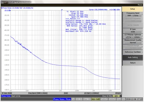
Figure 5-1: Phase noise measurement on the Keysight E5052B using auto-setup. DUT: SiT9365 differential oscillator via balun
5.2 Setting Input Attenuation
Input attenuation must be set according to the instrument vendor's recommendations. Excessive attenuation can reduce signal power to the point where thermal noise begins to raise the measurement floor. Too little attenuation may overload the front end and produce poor results. Figure 5-2 illustrates how the measurement noise floor increases when the input attenuator is changed from the auto-setup choice of 0 dB to 20 dB and 30 dB.
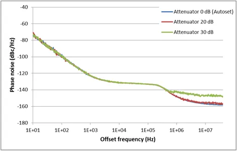
Figure 5-2: Effect of attenuator setting on phase noise measurement. Instrument: Keysight E5052B. DUT: SiT5356, 156.25 MHz.
5.3 Averaging
Most phase noise analyzers provide a measurement averaging feature. This runs the measurement the specified number of times and averages the results. Averaging smooths the phase noise trace but requires more time.
Figure 5-3 shows phase noise of a SiT5356 precision TCXO measured on the Keysight E5052B using two averaging settings: no averaging and 16x averaging. Users should try several averaging settings to find the best balance between measurement speed and quality.
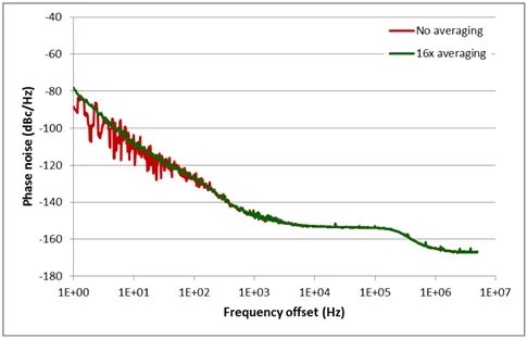
Figure 5-3: Phase noise measured with no averaging and with 16x averaging. Instrument: Keysight E5052B. DUT: SiT5356, 10 MHz
Both traces in Figure 5-3 are smooth and nearly identical at large offsets, but the trace without averaging appears noisy near the carrier. This difference arises from how the E5052B processes data. The analyzer collects raw phase data at a high sampling rate. Computing an FFT on the full dataset requires substantial computation, so the instrument splits the phase noise plot into fixed segments. This allows different resolutions for each segment so that small offsets can have higher resolution while distant offsets have lower resolution. For example, 1 Hz to 47.7 Hz might be the first segment, 47.7 Hz to 190.7 Hz the next, and so on. To compute an FFT for the first segment, the full time length of the raw data is used but the sampling rate is reduced by skipping samples. For the next segment, the sampling rate is higher than the first segment but the sequence duration is reduced.
This approach also enables another benefit. For higher-frequency segments, the data used for FFT may have the maximum sampling rate but relatively short duration. The raw phase dataset can be split into multiple consecutive datasets corresponding to these segments. FFTs can then be computed separately for each dataset and averaged to obtain better segment results. In phase noise analyzer documentation, this process is described as performing a number of correlations because multiple vector averages are effectively performed. The Keysight E5052 manual specifies how many correlations are applied to each phase noise segment. This extra processing is performed automatically by the instrument and cannot be adjusted by the user. That is why phase noise traces measured with the E5052B look smooth at higher offsets but still benefit from averaging to improve near-carrier measurement quality.
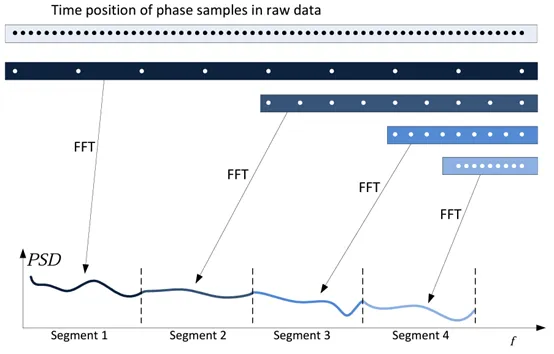
Figure 5-4: Stitching of segments in a phase noise plot
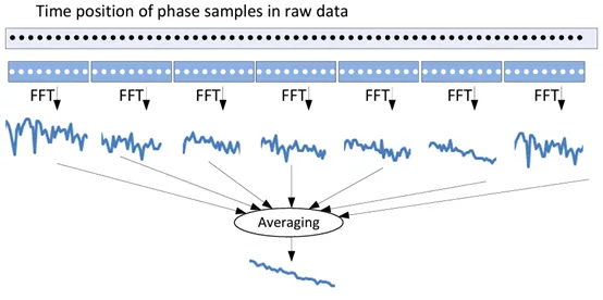
Figure 5-5: Higher-frequency segments contain enough data to perform multiple correlations and average the results
5.4 Cross Correlation
Cross correlation is another technique to improve the measurement noise floor. The DUT signal connected to the phase noise analyzer is split into two measurement channels, each with its own reference and PLL. Cross correlation is applied between the outputs of these two channels. Noise that originates in the DUT is coherent and therefore unaffected by cross correlation. Noise from the measurement channels is incoherent and is reduced by the cross-correlation operation by a factor of sqrt(M), where M is the number of correlations.
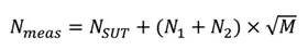
where L(f) is the spurious level in dBc and f_carrier is the carrier frequency.
In Figure 5-9, the largest spur is about -100 dBc, a typical performance for the SiTime SiT9365 differential oscillator. Converting this to RMS jitter yields a spur-related contribution of only 14.4 fs RMS.
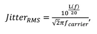
So the spur contributes only 14.4 fs RMS
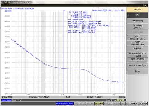
Figure 5-8: Phase noise measured with spurs removed (spur modes ignored). Instrument: Keysight E5052B. DUT: SiT9365, 156.25 MHz
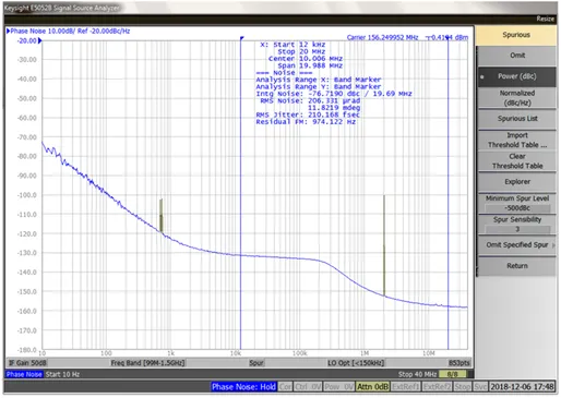
Figure 5-9: Phase noise measured with detected spurs displayed in dBc (power spur mode). Instrument: Keysight E5052B. DUT: SiT9365, 156.25 MHz