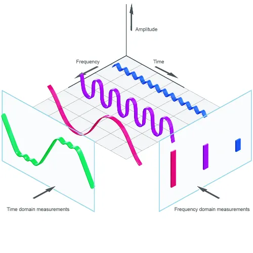
Relationship Between Frequency and Time Domains
Technical overview of frequency-domain and time-domain signal analysis, transforms (Fourier/Laplace), measurements (spectrum, TDR) and VNA-based time-domain conversions.
In the rapidly evolving field of electronics, RF & Wireless Technology stands as a cornerstone for modern connectivity and communication systems. This category delves into the principles and applications of radio frequency (RF) engineering and wireless protocols, essential for designing efficient printed circuit boards (PCBs) that power everything from smartphones to satellite systems. As devices become increasingly interconnected, understanding RF fundamentals ensures reliable signal transmission, minimal interference, and optimal performance in diverse environments. Our collection of articles offers comprehensive guides on RF circuit design, including antenna selection, impedance matching, and signal modulation techniques. Tutorials provide step-by-step instructions for implementing wireless standards such as Wi-Fi, Bluetooth, and 5G, while insights explore emerging trends like IoT integration and millimeter-wave technologies. Best practices focus on troubleshooting common issues, such as electromagnetic compatibility and power efficiency, helping engineers avoid pitfalls in real-world projects. The practical value of RF & Wireless Technology extends to numerous industries, from telecommunications and automotive systems to healthcare devices and smart cities. By mastering these concepts, professionals can develop innovative solutions that enhance data transfer speeds, extend battery life, and support seamless connectivity. Whether you are optimizing PCB layouts for high-frequency operations or evaluating wireless security measures, the knowledge here equips you to tackle complex challenges with confidence. Readers will find value in browsing through these resources to gain a deeper understanding of how RF principles drive technological advancements. Each article builds on core concepts, offering actionable advice that bridges theory and practice for engineers at all levels.
Technical overview of frequency-domain and time-domain signal analysis, transforms (Fourier/Laplace), measurements (spectrum, TDR) and VNA-based time-domain conversions.
Overview of RF filters in RFFE design: duplexing, isolation, selectivity, and antenna multiplexers for coexistence, receiver sensitivity, and compact wireless devices.
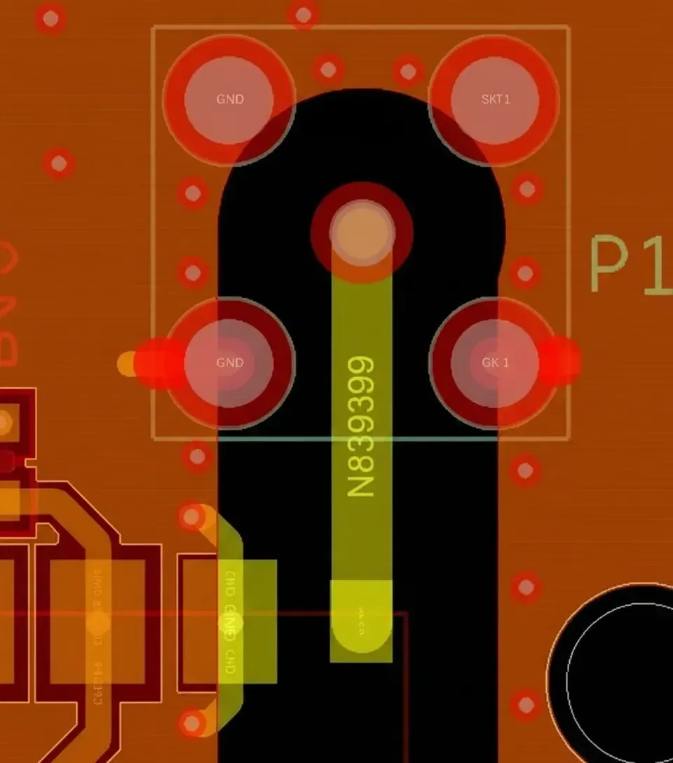
Improve antenna PCB design and integration for wireless systems. This guide covers radiation patterns, impedance matching, and material choice for reliable RF and 5G performance.
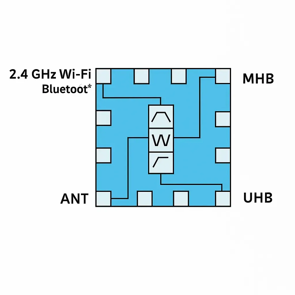
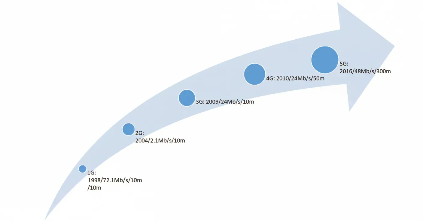
Technical analysis of a smartphone RF PCB and antenna integration, listing supported wireless systems and frequency ranges: cellular bands (2G–5G), Wi?Fi, Bluetooth, UWB, GNSS.
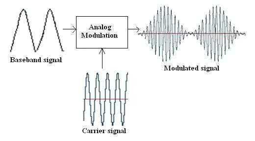
Learn expert techniques for RF modulation PCB design and manufacturing. This article covers signal integrity, impedance control, and material choice for reliable wireless communication.
Analysis of single-chip Bluetooth CMOS architecture vs multi-chip designs, detailing VCO, IF receiver, RF front-end and integration advantages for cost and PCB size.
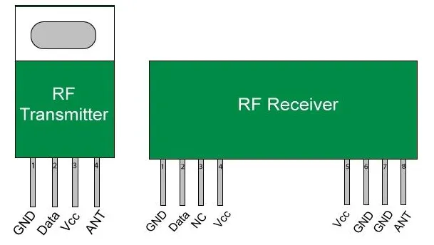
Overview of RF receiver systems: key metrics (sensitivity, noise figure), circuit structure, and design/test strategies to improve demodulation and interference rejection.
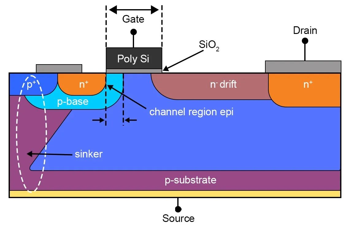
Overview of RF circuits, components (amplifier, filter, mixer, coupler, transceiver) and the roles of MOS devices in amplification, switching, oscillation and frequency conversion.
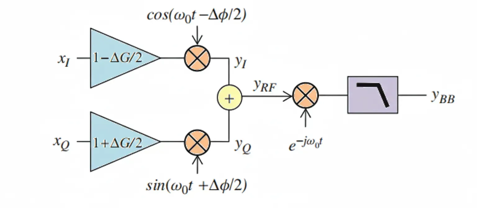
Overview of RF impairments in zero-/low-IF transceivers and digital calibration needs: thermal noise, sampling jitter, CFO/SFO, ADC effects; focus on phase noise and I/Q imbalance
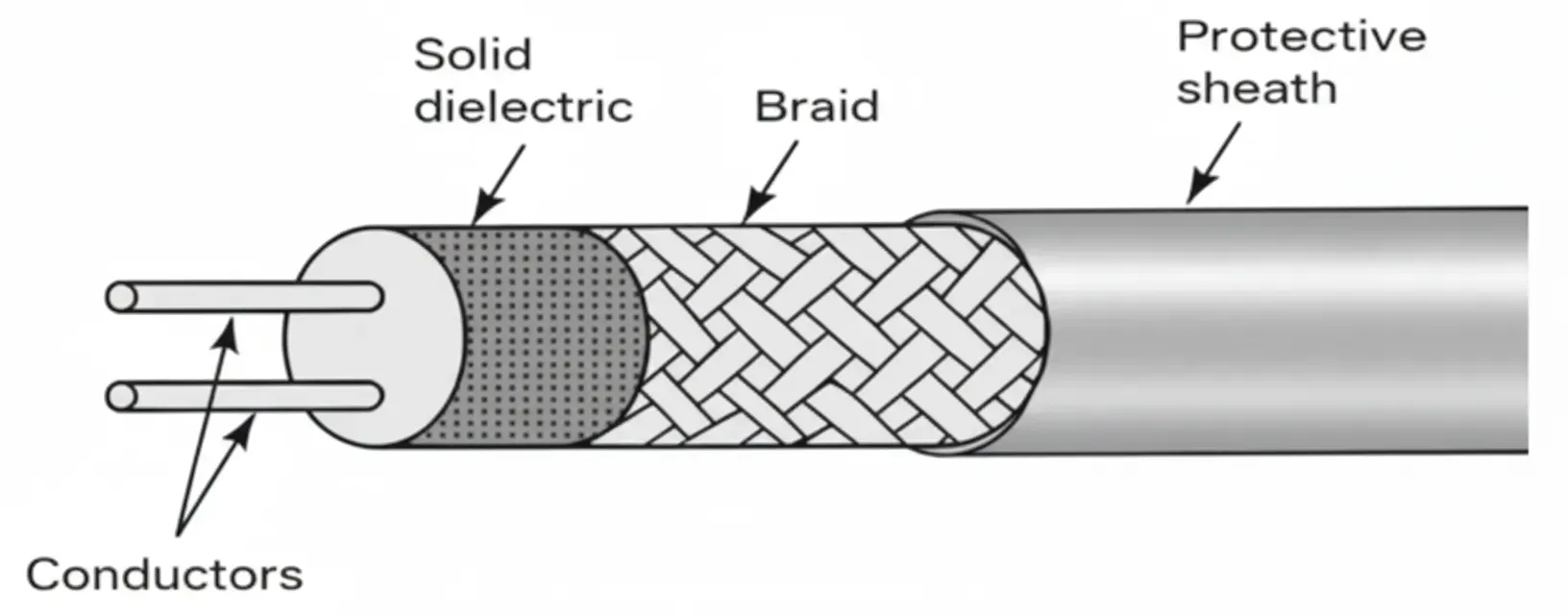
Technical overview of the parallel-wire transmission line: construction, characteristic impedance, balanced operation, losses and why coaxial cable replaced it.
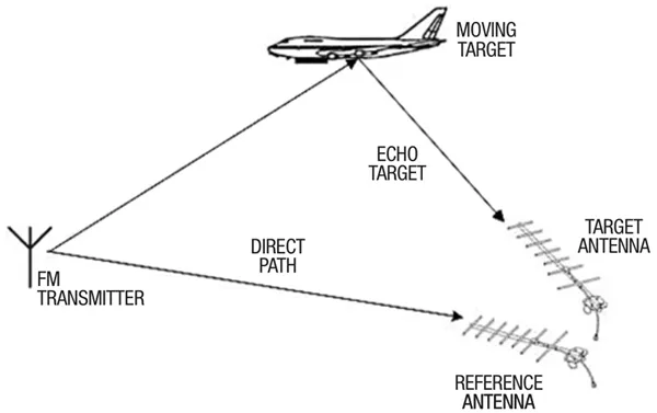
Technical overview of passive radar receiver tasks (detection, PDW extraction, identification, tracking) and architectures, highlighting channelized and microwave photonic receivers.
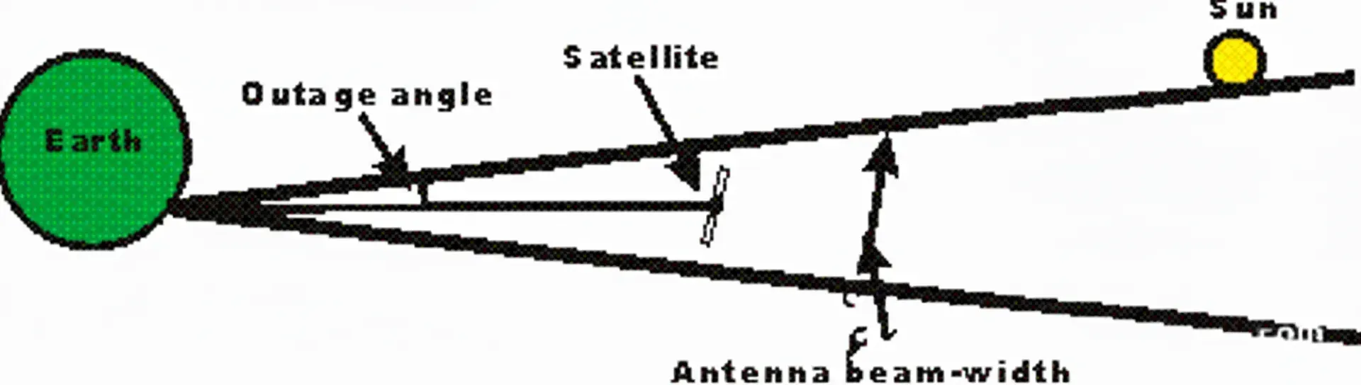
Understand satellite sun outage causes, timing around equinoxes, beamwidth effects, and RF noise impact. Explore receiver electronics design, low-noise amplification, PCB material selection, and reliability considerations for satellite ground stations and communication systems.