Voice interfaces have become a cornerstone of modern consumer electronics, powering devices from smart speakers and wearables to home appliances and automotive systems. Speech recognition (automatic speech recognition or ASR) and speech synthesis enable natural human-machine interaction, while offline and cloud-hybrid implementations balance performance, latency, and privacy. From a PCB manufacturing perspective, these systems impose strict requirements on layout, signal integrity, power distribution, thermal management, and component integration. High-quality PCBs are essential to capture clean audio signals, process them efficiently, and deliver reliable voice responses.
Core Principles of Speech Recognition and PCB Implications
Speech recognition converts acoustic signals into text or commands through a pipeline of preprocessing, feature extraction, acoustic modeling, language modeling, and decoding. The process begins with microphone capture of audio, followed by analog and digital processing on the PCB.
Key stages include:
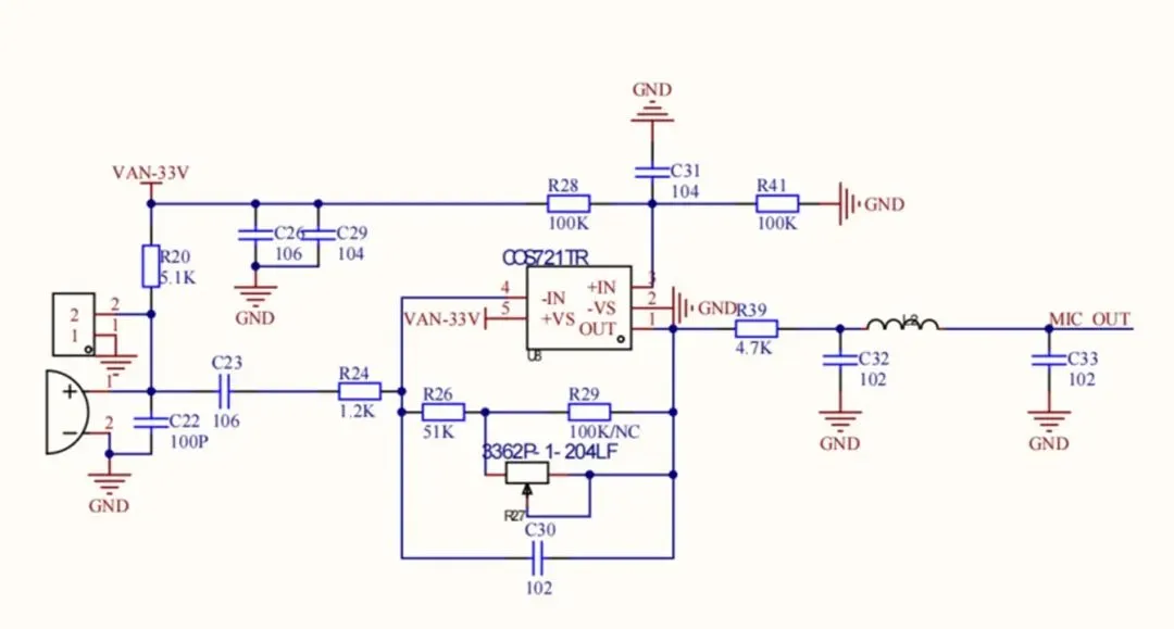
- Acoustic signal preprocessing: Filtering, sampling, framing, and endpoint detection remove noise and prepare the signal. On consumer electronics PCBs, this relies on precise analog front-end circuits, including band-pass filters to isolate the human speech band (typically 300–3400 Hz) and suppress power-line interference. Proper PCB layout minimizes crosstalk and ensures stable signal-to-noise ratio (SNR) through careful grounding and trace routing.
- Feature extraction: Techniques such as Mel-frequency cepstral coefficients (MFCC) or linear predictive cepstral coefficients (LPCC) transform time-domain signals into frequency-domain features. These computations benefit from low-noise PCB environments and strategic placement of ADCs near microphones to preserve signal fidelity.
- Acoustic and language models: Traditional GMM-HMM systems have largely given way to DNN-HMM or end-to-end deep learning architectures. Hardware acceleration for these models—via integrated DSPs or MCUs—requires PCBs with adequate power delivery networks and thermal relief to handle computational loads without throttling.
Effective PCB design directly impacts recognition accuracy by reducing noise, electromagnetic interference (EMI), and signal degradation that could otherwise corrupt feature vectors or model outputs.
Speech Synthesis in Voice Assistants: TTS and PCB Considerations
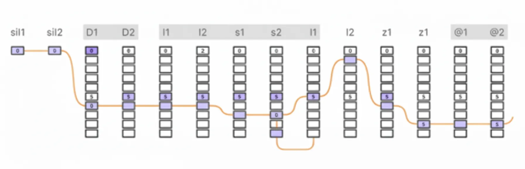
Speech synthesis (text-to-speech or TTS) complements recognition by generating natural-sounding responses. Systems like Siri employ hybrid unit selection combined with deep learning, using mixture density networks (MDNs) to predict prosodic features such as pitch, duration, and spectral characteristics. This enables fluent, human-like output from recorded voice units.

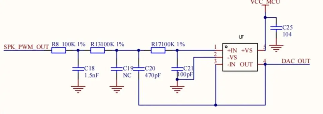
On the PCB side, synthesis demands clean digital-to-analog conversion and amplification paths. Low-jitter clocks, optimized power planes, and minimal trace lengths between processors and audio codecs are critical to avoid audible artifacts. In compact consumer devices, multilayer PCBs with controlled impedance support high-speed data movement between memory, MCUs, and audio output stages while managing heat from continuous processing.
Offline Voice Recognition: MCU-Based Implementations and Hardware Integration
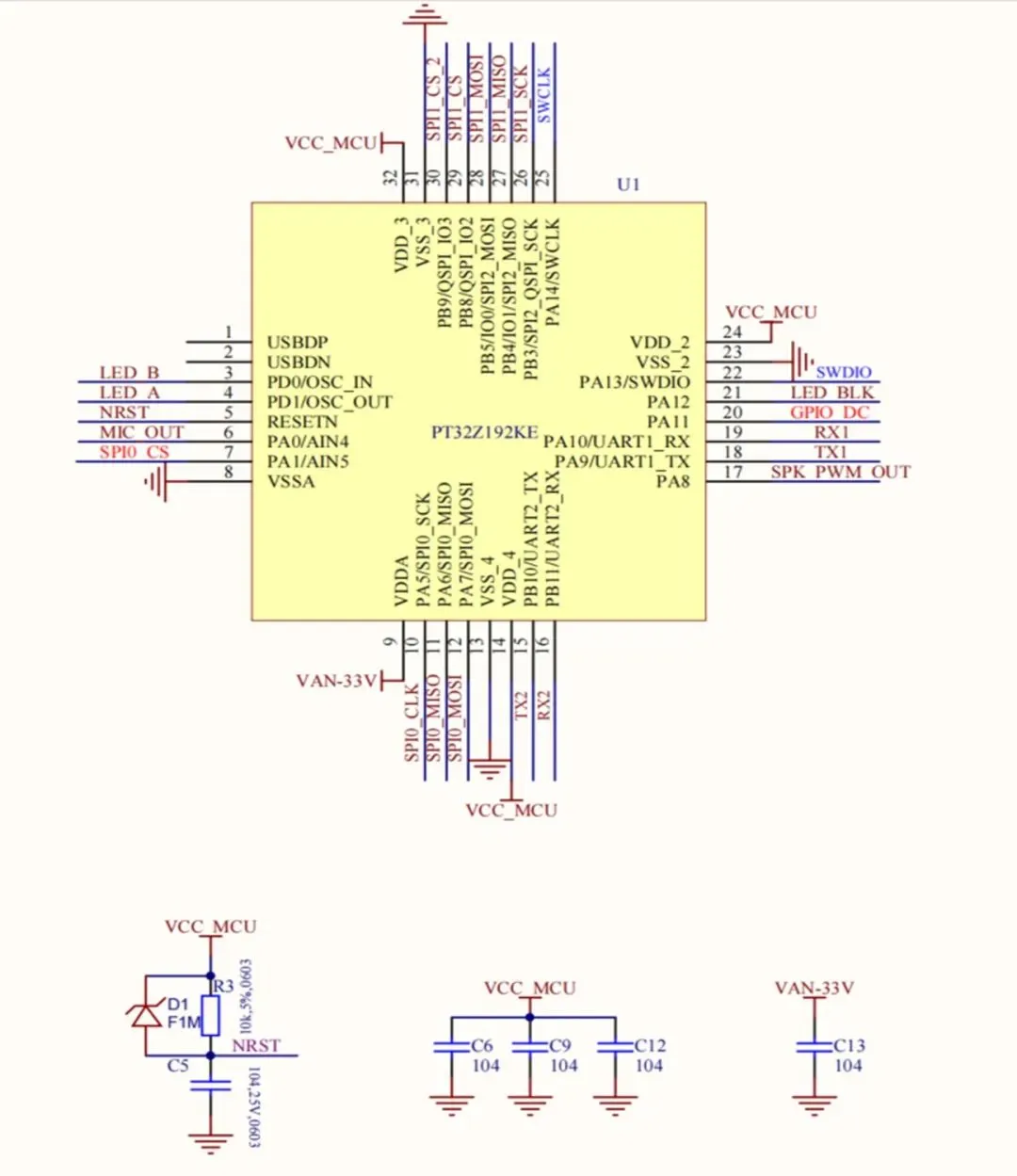
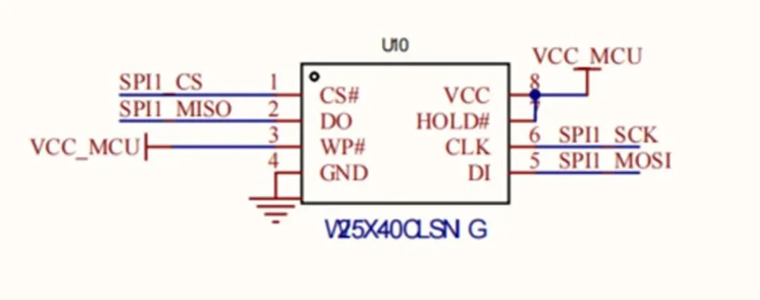
Offline solutions enable local processing without cloud dependency, reducing latency, cost, and power consumption. Platforms built around Cortex-M3 MCUs (such as the PT32Z192 running at 160 MHz with 512 KB Flash and 128 KB RAM) integrate high-precision 12-bit ADCs, timers for PWM audio, and interfaces like UART, I2C, and SPI.
PCB design for these systems focuses on:
- High-sensitivity microphone circuits with proper shielding and decoupling.
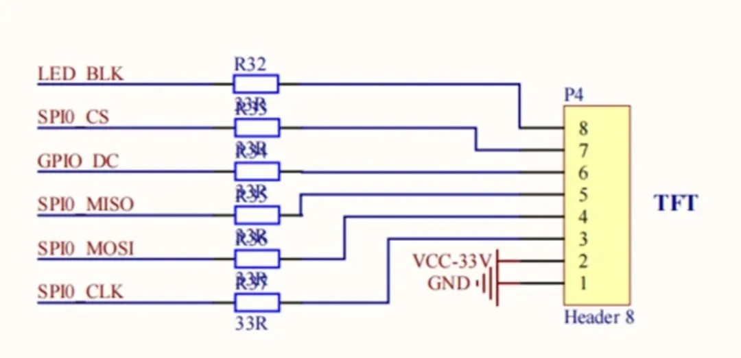
- Compact layouts supporting TFT displays via SPI and optional NOR Flash or dedicated voice playback chips.
- PWM-based audio output or dedicated playback ICs, requiring robust power amplification stages and careful trace routing to minimize distortion.
- Expansion ports for wireless modules (Bluetooth, Zigbee, etc.).
These designs target applications like voice-controlled lighting, fans, and smart home devices, where recognition distances up to 10 meters in quiet environments depend on clean analog paths and efficient digital processing on the PCB.
Amazon Echo Architecture: Microphone Arrays, DSP, and System-Level PCB Challenges
Smart speakers like the Amazon Echo and Echo Dot illustrate advanced voice control hardware. Teardowns reveal integrated application processors (e.g., TI DM3725 with ARM Cortex-A8 and DSP), connectivity solutions, LPDDR RAM, and eMMC storage. A hallmark is the 7-microphone array using MEMS microphones with beamforming for far-field capture and noise rejection—even during music playback.
PCB implications include:
- Dense microphone array layouts requiring matched trace lengths, impedance control, and isolation to support beamforming algorithms.
- DSP integration for real-time filtering, echo cancellation, and pattern matching, demanding efficient power distribution and thermal vias.
- Hybrid local/cloud processing, where the PCB must reliably handle both simple wake-word detection locally and high-bandwidth data offloading via Wi-Fi/Bluetooth modules.
- Component choices (processors, memory) influence manufacturability, with emphasis on supply chain stability and cost optimization during volume production.
Key PCB Engineering Challenges in Voice Systems
Voice-enabled consumer electronics face several recurring PCB constraints:
- Signal integrity and EMI/EMC: Microphone arrays and high-speed digital lines (DSP, MCUs) are sensitive to noise. Techniques include star grounding, guard traces, and proper stack-up design (e.g., FR4 with adequate copper weight for power planes).
- Thermal management: Continuous audio processing and wireless activity generate heat in compact enclosures. High-Tg materials, thermal vias, and copper pours help maintain performance and reliability.
- Power integrity: Multiple voltage rails for analog, digital, and RF sections require careful decoupling and low-impedance paths to prevent audio artifacts or recognition errors.
- Miniaturization and HDI: Multi-layer and high-density interconnect (HDI) PCBs enable integration of MEMS microphones, processors, and memory in small form factors while supporting fine-pitch components.
- Reliability: Consumer devices must withstand temperature cycling, vibration, and humidity. Robust via design, solder mask quality, and material selection (e.g., low-loss dielectrics where needed) reduce failure rates.
Manufacturing considerations include tight tolerances on impedance-controlled traces, precise drilling for vias near sensitive analog sections, and panelization strategies that maintain signal quality across production batches.
Applications and Manufacturing Best Practices
These PCB principles apply across automotive infotainment, industrial controls, medical devices, and consumer smart home products. For high-volume production, partnering with experienced PCB manufacturers ensures optimized stack-ups, material selection, and assembly processes that meet both performance and cost targets.
By prioritizing signal integrity, thermal performance, and manufacturability from the schematic stage onward, engineers can deliver voice systems that combine high recognition accuracy with long-term reliability.
Future Trends in PCB-Enabled Voice Technologies
The rapid evolution of voice interfaces is driving several PCB-centric advancements. On-device AI acceleration through specialized neural processing units (NPUs) and edge AI chips will demand higher-layer-count PCBs with improved thermal dissipation and finer-pitch routing to support real-time inference without cloud latency. Integration with 5G and emerging 6G networks will require PCBs optimized for high-frequency RF performance, including low-loss materials and precise impedance control for hybrid cloud-edge voice processing.
Miniaturization trends favor rigid-flex and flexible PCBs, enabling voice capabilities in wearables, hearables, and ultra-thin devices while maintaining signal integrity across bending zones. Sustainability pressures are pushing manufacturers toward halogen-free laminates, recyclable substrates, and lead-free processes that still meet stringent thermal and electrical requirements. Advanced packaging techniques such as chiplets and 3D integration will influence stack-up design, via-in-pad technology, and thermal management strategies.
Emerging microphone technologies—including larger arrays, ultrasonic sensing, and AI-enhanced beamforming—will further increase the need for low-noise analog paths, matched impedance routing, and robust EMI shielding on the PCB. Hardware security modules integrated directly into the board will become standard to protect voice data and model integrity.
Conclusion
Speech recognition and voice control systems represent a sophisticated intersection of acoustics, machine learning, and hardware engineering. Success hinges on PCB design and manufacturing excellence that preserves signal fidelity, manages thermal and power constraints, and supports reliable high-volume production. As consumer electronics continue to embrace voice as a primary interface, manufacturers who master these PCB-level considerations will deliver superior user experiences with greater accuracy, lower power consumption, and enhanced durability. For optimized PCB solutions tailored to next-generation voice applications, collaboration with specialized manufacturers remains essential to translating innovative concepts into reliable, market-ready products.