


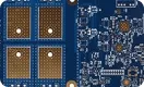


Some engineers feel that industry pays plenty of attention to signal integrity (SI) while power integrity (PI) does not always receive the same rigor. The perception often stems from experience in low-frequency applications, where switching power supplies are largely designed using established heuristics and simple functional simulations. In many medium- to low-frequency designs under 50–100 MHz, capacitor selection and placement rules of thumb generally work, and even vendor-provided spreadsheet tools can adequately cover this band.
For applications above 100 MHz, many assume the problem belongs primarily to the IC and has little to do with the board, leading to a belief that board-level PI simulation adds limited value unless it incorporates chip-to-chip solutions with package and silicon models. Is that really the case? In practice, there is a great deal PI can and should do at the board level.

Figure 1 | Perceived focus on SI versus PI in typical design flows

Figure 2 | Is pure board-level PI simulation meaningful without IC/package models?
There is significant constructive work to be done in power integrity. The sections below outline what SI and PI each cover, where they intersect, and how to make practical design decisions at the PCB level.
Signal Integrity and Power Integrity Fundamentals
Signal integrity and power integrity are related but distinct analysis domains concerned with the correct operation of digital circuits. SI focuses on ensuring that a logic ‘1’ transmitted by the driver is still seen as a ‘1’ at the receiver (and likewise for ‘0’), with acceptable waveform quality and timing. PI focuses on ensuring the power distribution network (PDN) can supply the instantaneous current demanded by drivers and receivers so they can switch and sample those logic levels correctly. In that sense, PI can be viewed as a prerequisite for SI, but practically they are complementary aspects of the same physical system.
Why Separate Analyses Are Necessary
If compute resources were unlimited and complete models existed, one might analyze the entire system as a whole and diagnose every issue in a single co-simulation. In reality, model scope, tool capabilities, and compute cost necessitate domain-specific analyses that target the most likely problems. SI analysis generally confines the scope to the link from transmitter to receiver and models the drivers, receivers, packages, PCB interconnects (traces, vias, discrete components, connectors), and their electromagnetic behavior.
In SI, the goal is to resolve signal quality, crosstalk, and timing issues. Driver and receiver models describe buffer impedance, edge rate, and voltage swing. IBIS or SPICE models are typically used and combined with interconnect models to evaluate the waveform at the receiver. Interconnects behave as transmission lines with characteristic impedance, delay, and loss. Their EM properties are solved with field solvers and represented as circuit elements or S-parameters for use in SI simulation.
Most traces can be modeled as uniform 2D cross-sections, sufficient for computing characteristic impedance and delay. This is often the starting point: define the layer stackup, dielectric thicknesses, and choose trace widths to achieve the target impedance. Vias are more challenging, and for faster signals their 3D behavior becomes critical. Gigabit-per-second signals require accurate 3D via models. Fortunately, such high-speed nets are usually limited in number, localizing their impact.
Fast single-ended signals passing through vias interact strongly with the PDN. Their return currents find paths through nearby stitching vias, decoupling capacitors, and plane pairs—the same PDN structures that PI models and optimizes.

Figure 3 | Energy propagation on a trace cross-section, through a signal via, and across the PDN. In PI, higher-frequency energy spreads across plane pairs in both x and y, making the analysis inherently more complex than a 1D transmission line. DC analysis is comparatively straightforward, requiring resistive modeling of traces, planes, and vias.
At higher frequencies, accurately predicting PDN impedance between power and ground at different locations requires distributed analysis. The impedance varies with component placement, mounting methods, capacitor type and value, and the stackup’s spreading inductance. Simple “lumped” decoupling analyses that treat the PDN as a single node are useful for early estimation—ensuring enough capacitance of reasonable values—but distributed analysis is needed to confirm impedance targets across the board.
Signal Integrity Simulation
SI simulation addresses three key issues in high-speed signals: signal quality, crosstalk, and timing. For signal quality, the goal is to obtain clean edges without excessive overshoot or undershoot and with controlled ringing. Termination is the primary tool: matching the driver’s output impedance to the line impedance reduces reflections. In multi-drop topologies it may be impossible to perfectly match, so termination choice, topology, and stub length require co-optimization to prevent reflections from degrading signal quality and timing.

Figure 4 | Using SI analysis and design space exploration to eliminate signal quality and crosstalk issues
Propagation delay through the PCB is another output of SI simulation; it depends on route length, propagation velocity, and the receiver’s threshold crossing time, which is determined by the waveform shape. These results drive routing length constraints and inter-pair skew budgets. Crosstalk simulations consider multiple coupled transmission lines to quantify near-end and far-end coupling as traces are crowded. Results guide minimum spacing rules and shielding strategies.
Power Integrity Simulation
PI analysis commonly includes DC IR drop, decoupling, and noise analyses. DC IR drop evaluates the voltage lost to resistive paths in complex trace and plane geometries, identifying whether loads still see adequate voltage under worst-case currents. It also identifies regions of high current density, which can be co-simulated with thermal tools to assess hotspots.

Figure 5 | Current density and temperature maps showing hotspots in PI/thermal co-simulation. A common remedy for excessive IR drop or hot spots is to add metal—wider or thicker traces and planes, extra plane layers, or additional vias.
Decoupling analysis focuses on minimizing PDN impedance between power and ground at IC locations and across frequency. It drives changes in capacitor values, types, and counts; requires capacitor models that include parasitic inductance and resistance; and often prompts changes in mounting and stackup to meet low impedance targets. Noise analysis covers how supply noise propagates across the board from the IC power pins and how well decoupling suppresses it. It also examines coupling between vias and characterizes simultaneous switching noise (SSN) driven by many outputs switching together. These analyses guide changes to the PDN planes, traces, capacitors, and stitching vias.
SI/PI Interaction Through the PDN and Vias
The PDN not only supplies current to ICs; it also serves as the return path for signals. The SI/PI overlap is most apparent at vias. For single-ended signals transitioning layers, the PDN provides the return current path, with nearby stitching vias or capacitors enabling the return to move between plane pairs. Consequently, the PDN sets the via’s impedance and delay characteristics, which must be modeled accurately for faster single-ended interfaces such as DDR3 and DDR4. The same combined SI/PI via model can quantify coupling from one via to another, as well as coupling from a signal via into the PDN.
PDN design is also critical for minimizing SSN. If the PDN impedance at the IC power pins is too high, the simultaneous switching currents generate a voltage that can modulate the signals themselves. A well-designed low-impedance PDN, established via decoupling analysis and verified by distributed simulations, suppresses these effects. While SPICE driver models have traditionally been used to include PDN effects in SI simulations, modern IBIS models also support mechanisms to incorporate PDN interactions during SI analysis.
SI and PI analyses are both indispensable for successful high-speed digital design. They provide actionable insight into necessary design changes. With improving models and compute capabilities, combined SI/PI simulation reveals how the circuit actually behaves, the true margins present in the design, and how to extract the best possible performance.
Practical Power Integrity Design Considerations
1. Power-System Noise Margin Analysis
Most ICs specify an acceptable supply voltage range, often ±5%. Many older regulators achieve output accuracy around ±2.5%, so the allowable peak-to-peak supply noise must fit within the remaining margin. Accuracy depends on conditions (load, temperature, etc.), so keep conservative margin.
2. Example: Calculating Power Noise Margin
Suppose an IC’s valid supply range is 3.13 V to 3.47 V, with a nominal 3.3 V rail. After assembly, the regulator outputs 3.36 V on the board. The available headroom to the upper limit is 3.47 - 3.36 = 0.11 V = 110 mV. If the regulator accuracy is ±1%, that is ±33.6 mV at 3.36 V. The remaining noise margin is approximately 110 ? 33.6 = 76.4 mV.
3. Where Power Noise Comes From
- Regulator ripple: The regulator output is not perfectly constant; some ripple is inherent.
- Finite control-loop response: Regulators cannot respond instantaneously to rapid load changes. They sense output deviation and adjust current to restore the setpoint, introducing transient error.
- Impedance in the supply and ground paths: Transient load currents flowing through the PDN’s resistance and inductance cause voltage drops. Package pins, pads, and interconnects introduce parasitic inductance; as transient current flows through these elements, the voltage at the IC’s power pins fluctuates.
4. Two Ways to Understand Decoupling
Decoupling capacitors are the primary means to mitigate power noise. They improve transient response and reduce PDN impedance.
4.1 Energy-Storage View
Boards place capacitors near the load IC’s power pins to act as local energy reservoirs. When the load current is steady, the regulator supplies the current (I0) and the capacitor current (Ic) is approximately zero, with the capacitor charged to the supply voltage. When the load steps, the regulator cannot instantaneously increase its output current, so the capacitor supplies the deficit. As the capacitor voltage changes, it delivers current to hold the IC’s supply voltage. With adequate capacitance, only a small voltage droop is needed to deliver a large transient current, stabilizing the local supply during the event.

Figure 6 | Decoupling capacitor as a local energy source to support transient load current
4.2 Impedance View
Now view the composite supply (regulator plus decoupling network) as seen from the load pads A–B. The goal is to keep the voltage at A–B nearly constant regardless of transient current. Equivalently, the PDN impedance Z seen by the load must be low across frequency so that ΔV remains small for any ΔI.

Figure 7 | Viewing the regulator and decoupling network as a composite supply at nodes A–B
This composite can be represented as an equivalent source with a finite output impedance. Adding decoupling effectively lowers the PDN’s AC impedance because capacitors present low impedance to AC (|Zc| = 1/ωC when ideal). In practice, the fundamental design principle for PDNs is to minimize impedance across the relevant frequency range using capacitors, low-inductance mounting, and appropriate plane geometry.

Figure 8 | Equivalent source model of the composite supply with finite output impedance

Figure 9 | Relationship between ΔV, ΔI, and Z highlights why a low PDN impedance is essential
5. Characteristics of Real Capacitors
There is no ideal capacitor in practice; “a capacitor is not just C.” Real capacitors include equivalent series resistance (ESR) and equivalent series inductance (ESL). These parasitics are negligible at low frequency but dominate at high frequency. ESL delays capacitor current changes and raises the effective impedance at high frequency. The self-resonant frequency (SRF) marks the transition from capacitive to inductive behavior; above SRF the device behaves inductively and its decoupling effectiveness drops.

Figure 10 | Practical capacitor SPICE model with ESR and ESL
ESL depends on construction and package size. Smaller packages and wide-body terminations typically offer lower ESL. Boards often include large capacitors such as tantalum or electrolytics for low-frequency energy storage. These parts tend to have higher ESR (lower Q), which broadens their effective frequency range and makes them suitable for board-level filtering. Higher-Q networks have sharper resonance and stronger peaking; in decoupling, a mix of values and Q factors helps cover a broader band without excessive peaking.
6. Local Decoupling Design
Digital logic must see supply voltages that keep logic levels within valid thresholds. For a 3.3 V logic family, for example, VIH may be above 2 V and VIL below 0.8 V depending on the standard. Place decoupling capacitors as close as possible between the IC’s power and ground pins. Under normal operation, they are charged and store energy. During switching, they provide the transient current locally so VCC and ground parasitics see minimal current during the edge, reducing induced voltage across those inductances. Using multiple capacitors in parallel reduces effective ESL and the loop impedance of the charge/discharge path. Pay attention to selection, placement, mounting distance, and mounting method; all of these strongly influence high-frequency impedance.
Combined, these SI and PI practices yield robust links and low-noise supplies. In modern high-speed designs, neither domain can be treated in isolation; their interaction through the PDN and the return paths makes co-optimization essential.